2.4: Integrated Rate Laws

Last updated
Save as PDF

Page ID: 101148

$ \newcommand{\vecs}[1]{\overset { \scriptstyle \rightharpoonup} {\mathbf{#1}} } $

$ \newcommand{\vecd}[1]{\overset{-\!-\!\rightharpoonup}{\vphantom{a}\smash {#1}}} $

$ \newcommand{\id}{\mathrm{id}}$ $ \newcommand{\Span}{\mathrm{span}}$

( \newcommand{\kernel}{\mathrm{null}\,}\) $ \newcommand{\range}{\mathrm{range}\,}$

$ \newcommand{\RealPart}{\mathrm{Re}}$ $ \newcommand{\ImaginaryPart}{\mathrm{Im}}$

$ \newcommand{\Argument}{\mathrm{Arg}}$ $ \newcommand{\norm}[1]{\| #1 \|}$

$ \newcommand{\inner}[2]{\langle #1, #2 \rangle}$

$ \newcommand{\Span}{\mathrm{span}}$

$ \newcommand{\id}{\mathrm{id}}$

$ \newcommand{\Span}{\mathrm{span}}$

$ \newcommand{\kernel}{\mathrm{null}\,}$

$ \newcommand{\range}{\mathrm{range}\,}$

$ \newcommand{\RealPart}{\mathrm{Re}}$

$ \newcommand{\ImaginaryPart}{\mathrm{Im}}$

$ \newcommand{\Argument}{\mathrm{Arg}}$

$ \newcommand{\norm}[1]{\| #1 \|}$

$ \newcommand{\inner}[2]{\langle #1, #2 \rangle}$

$ \newcommand{\Span}{\mathrm{span}}$ $ \newcommand{\AA}{\unicode[.8,0]{x212B}}$

$ \newcommand{\vectorA}[1]{\vec{#1}} % arrow$

$ \newcommand{\vectorAt}[1]{\vec{\text{#1}}} % arrow$

$ \newcommand{\vectorB}[1]{\overset { \scriptstyle \rightharpoonup} {\mathbf{#1}} } $

$ \newcommand{\vectorC}[1]{\textbf{#1}} $

$ \newcommand{\vectorD}[1]{\overrightarrow{#1}} $

$ \newcommand{\vectorDt}[1]{\overrightarrow{\text{#1}}} $

$ \newcommand{\vectE}[1]{\overset{-\!-\!\rightharpoonup}{\vphantom{a}\smash{\mathbf {#1}}}} $

$ \newcommand{\vecs}[1]{\overset { \scriptstyle \rightharpoonup} {\mathbf{#1}} } $

$ \newcommand{\vecd}[1]{\overset{-\!-\!\rightharpoonup}{\vphantom{a}\smash {#1}}} $

$\newcommand{\avec}{\mathbf a}$ $\newcommand{\bvec}{\mathbf b}$ $\newcommand{\cvec}{\mathbf c}$ $\newcommand{\dvec}{\mathbf d}$ $\newcommand{\dtil}{\widetilde{\mathbf d}}$ $\newcommand{\evec}{\mathbf e}$ $\newcommand{\fvec}{\mathbf f}$ $\newcommand{\nvec}{\mathbf n}$ $\newcommand{\pvec}{\mathbf p}$ $\newcommand{\qvec}{\mathbf q}$ $\newcommand{\svec}{\mathbf s}$ $\newcommand{\tvec}{\mathbf t}$ $\newcommand{\uvec}{\mathbf u}$ $\newcommand{\vvec}{\mathbf v}$ $\newcommand{\wvec}{\mathbf w}$ $\newcommand{\xvec}{\mathbf x}$ $\newcommand{\yvec}{\mathbf y}$ $\newcommand{\zvec}{\mathbf z}$ $\newcommand{\rvec}{\mathbf r}$ $\newcommand{\mvec}{\mathbf m}$ $\newcommand{\zerovec}{\mathbf 0}$ $\newcommand{\onevec}{\mathbf 1}$ $\newcommand{\real}{\mathbb R}$ $\newcommand{\twovec}[2]{\left[\begin{array}{r}#1 \\ #2 \end{array}\right]}$ $\newcommand{\ctwovec}[2]{\left[\begin{array}{c}#1 \\ #2 \end{array}\right]}$ $\newcommand{\threevec}[3]{\left[\begin{array}{r}#1 \\ #2 \\ #3 \end{array}\right]}$ $\newcommand{\cthreevec}[3]{\left[\begin{array}{c}#1 \\ #2 \\ #3 \end{array}\right]}$ $\newcommand{\fourvec}[4]{\left[\begin{array}{r}#1 \\ #2 \\ #3 \\ #4 \end{array}\right]}$ $\newcommand{\cfourvec}[4]{\left[\begin{array}{c}#1 \\ #2 \\ #3 \\ #4 \end{array}\right]}$ $\newcommand{\fivevec}[5]{\left[\begin{array}{r}#1 \\ #2 \\ #3 \\ #4 \\ #5 \\ \end{array}\right]}$ $\newcommand{\cfivevec}[5]{\left[\begin{array}{c}#1 \\ #2 \\ #3 \\ #4 \\ #5 \\ \end{array}\right]}$ $\newcommand{\mattwo}[4]{\left[\begin{array}{rr}#1 \amp #2 \\ #3 \amp #4 \\ \end{array}\right]}$ $\newcommand{\laspan}[1]{\text{Span}\{#1\}}$ $\newcommand{\bcal}{\cal B}$ $\newcommand{\ccal}{\cal C}$ $\newcommand{\scal}{\cal S}$ $\newcommand{\wcal}{\cal W}$ $\newcommand{\ecal}{\cal E}$ $\newcommand{\coords}[2]{\left\{#1\right\}_{#2}}$ $\newcommand{\gray}[1]{\color{gray}{#1}}$ $\newcommand{\lgray}[1]{\color{lightgray}{#1}}$ $\newcommand{\rank}{\operatorname{rank}}$ $\newcommand{\row}{\text{Row}}$ $\newcommand{\col}{\text{Col}}$ $\renewcommand{\row}{\text{Row}}$ $\newcommand{\nul}{\text{Nul}}$ $\newcommand{\var}{\text{Var}}$ $\newcommand{\corr}{\text{corr}}$ $\newcommand{\len}[1]{\left|#1\right|}$ $\newcommand{\bbar}{\overline{\bvec}}$ $\newcommand{\bhat}{\widehat{\bvec}}$ $\newcommand{\bperp}{\bvec^\perp}$ $\newcommand{\xhat}{\widehat{\xvec}}$ $\newcommand{\vhat}{\widehat{\vvec}}$ $\newcommand{\uhat}{\widehat{\uvec}}$ $\newcommand{\what}{\widehat{\wvec}}$ $\newcommand{\Sighat}{\widehat{\Sigma}}$ $\newcommand{\lt}{<}$ $\newcommand{\gt}{>}$ $\newcommand{\amp}{&}$ $\definecolor{fillinmathshade}{gray}{0.9}$

Learning Objectives

By the end of this section, you should be able to:

Determine the reaction order and rate constant from kinetic data using the linearized form of integrated rate laws

Integrated Rate Laws

Rate laws are differential equations that can be integrated to find how the concentrations of reactants and products change with time. We can imagine a fairly complex system with multiple reactions described by

\[𝑟_{1}=𝑘_{𝑟1}∗𝑓(𝐴,𝐵,...), 𝑟_{2}=𝑘_{𝑟2}∗𝑓(𝐴,𝐵,...), 𝑟_{3}, 𝑟_{4}...\]

The concentration of all components can be described by equations such as $\frac{d[A]}{dt}=−r_{1}−2r_{2}...$ We need to integrate these to find concentrations at a given time.

Any of these rate laws can be solved numerically (you’ll learn about this in CHBE 230), but some simpler cases can also be solved analytically.

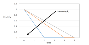
Zeroth Order Reactions

A zeroth-order reaction is one whose rate is independent of concentration$^{[1]}$; Say we have a reaction:

\[A → B\]

It’s differential rate law would be represented as:

\[r = -\frac{d[A]}{dt} =k_{r}\]

Integrating from t=0, when the system has a concentration of A as $[A]_{0}$, to some time t, when the system has a concentration represented by $[A]$

\[\int_{[A]_{0}}^{[A]} \mathrm d[A] = \int_{t_{0}=0}^{t} \mathrm -k_{r}\]

$-[A]_{0}=-k_{r}*t$ or $[A]=[A]_{0}-k_{r}*t$

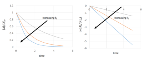
First-Order Reactions

Using a similar approach to the zeroth order reactions:

\[r=-\frac{d[A]}{dt}=k_{r}[A]\]

\[\int_{[A]_{0}}^{[A]} \frac{d[A]}{[A]} = \int_{t_{0}=0}^{t} \mathrm-k_{r}\]

$ln[A]-ln[A]_{0}=-k_{r}*t$ or $[A]=[A]_{0}e^{-k_{r}*t}$

Example: Half-life for First-order Reactions

text

Solution

text.

Based on the equation we derived, what is an expression for the time taken for half of A to be consumed (half-life)?

\[ln[A]-ln[A]_{0}=-k_{r}*t\]

\begin{align*}
k_{r}* t_{1/2} & = -ln \frac{[A]}{[A]_{0}} \\
& = -ln \frac{\frac{1}{2}[A]_{0}}{[A]_{0}} \\
& =-ln(\frac{1}{2}) \\
& = ln(2)
\end{align*}

$\text{[math]}$

Note that this half-life does not depend on [A].

Practice: use $[A]=[A]_{0}e^{-k_{r}*t}$, you should get the same result.

Solution

\begin{align*}
[A] & = [A]_{0}*e^{-k_{r}t_{1/2}} \\
\frac{[A]}{[A]_{0}}& = e^{-k_{r}t_{1/2}} \\
\frac{1}{2} & = e^{-k_{r}t_{1/2}} \\
ln(\frac{1}{2}) & = -k_{r}*t_{1/2}
\end{align*}

$\text{[math]}$

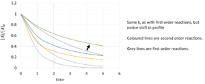
Second-Order Reactions

\[r=-\frac{d[A]}{dt}=k_{r}[A]^2\]

\[\int_{[A]_{0}}^{[A]} \frac{d[A]}{[A]^2} = \int_{t_{0}=0}^{t} \mathrm-k_{r}\]

$\frac{1}{[A]}-\frac{1}{[A]_{0}}=k_{r}*t$ or $[A]=\frac{[A]_{0}}{1+k_{r}*t*[A]_{0}}$

Using this to find half life, we find that: $\text{[math]}$

References

[1] Chemistry LibreTexts. 2020. 12.4 Integrated Rate Laws. [online] Available at: <https://chem.libretexts.org/Bookshelves/General_Chemistry/Book%3A_Chemistry_(OpenSTAX)/12%3A_Kinetics/12.4%3A_Integrated_Rate_Laws#:~:text=We%20measure%20values%20for%20the,different%20concentrations%20of%20the%20reactants.&text=Integrated%20rate%20laws%20are%20determined,various%20times%20during%20a%20reaction.> [Accessed 24 April 2020].

Search

Text Color

Text Size

Margin Size

Font Type

Example: Half-life for First-order Reactions

Solution