2.8: Steady-State Approximation

Learning Objectives

By the end of this section, you should be able to:

• Select the rate-determining step given the consecutive reactions and overall rate law of the reaction

Derive the rate law of a reaction given the consecutive reactions

Derive the rate law under pre-equilibria conditions

\[A\xrightarrow{\text{ka}}I\xrightarrow{\text{kb}}P\]

This approximation assumes intermediate, I, is in a low constant concentration,ie:

\[\frac{d[I]}{dt}=0\]

Generally the approximation is more accurate when \(k_{b}>>k_{a}\) (\(k_{b}\) is much greater than \(k_{a}\)). The bigger the difference, the more accurate the assumption.

\[k_{b}\]

As we saw before with first order reactions: \(\frac{d[A]}{dt}=-k_{a}[A]\) leads to \([A]=[A]_{0}e^{-k_{a}t}\)

Now: \(\frac{d[I]}{dt}=k_{a}[A]-k_{b}[I]≈0\) so \([I]=\frac{k_{a}}{k_{b}}[A]\)

For product: \(\frac{d[P]}{dt}=k_{b}[I]≈k_{a}[A]\) if we solved this, we would find: \([P]=[A]_{0}(1-e^{-k_{a}t})\)

Detailed proof: This is not required for the course, but might be useful for understanding.

For reactant:

\[\frac{d[A]}{dt}=-k_{a}[A]\]

\[[A]\]

\[[A]=constant*e^{-k_{a}t}\]

\[[A]=[A]_{0}*e^{-k_{a}t}\]

For intermediate:

\[\frac{d[I]}{dt}=k_{a}[A]-k_{b}[I]≈0\]

For product:

\[\frac{d[P]}{dt}=k_{b}[I]≈k_{a}[A]\]

\begin{align*}
\frac{d[P]}{dt} & = k_{a}[A] \\
\frac{d[P]}{dt} & = k_{a}*[A]_{0}*e^{-k_{a}t}\\
[P] & = \int k_{a}*[A]_{0}*e^{-k_{a}t}\\
[P] & = -[A]_{0}*e^{-k_{a}t} + constant
\end{align*}

To find the constant, we know that there is no product in the system, initially. At t=0, [P]=0. Subsitute t=0, the exponential term is equal to 1, so we are left with \(0=-[A]_{0}+constant\), so \(constant=[A]_{0}\), Therefore:

\[[P]= -[A]_{0}*e^{-k_{a}t} + [A]_{0}=[A]_{0}(1-e^{-k_{a}t})\]

Taking arbitrary values of \(k_{a}=1\) and \(k_{b}=10\), we can plot the concentration vs. time for all the components:

Exercise: Using Steady-state Approximation to Find Rate Law Expressions

To derive the overall rate law for this reaction:

\[2N_{2}O_{5(g)}→4NO_{2(g)}+O_{2(g)}\]

Assume the reaction follows the following three-step mechanism:

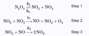
The final expression of the rate law should only contain \([N_{2}O_{5}]\) and the rate constants of the elementary steps.\(^{[1]}\)

Solution

Add example text here.

Step 1: Find the intermediates and express their rate of formation. Equate their rate of formation to 0 due to steady-state approximation.

\[\frac{d[NO]}{dt}=k_{2}[NO_{3}][NO_{2}]-k_{3}[NO_{3}][NO]=0\;\;\;\;\;(1)\]

\[\frac{d[NO_{3}]}{dt}=k_{f}[N_{2}O_{5}]-k_{b}[NO_{2}][NO_{3}]-k_{2}[NO_{3}][NO_{2}]-k_{3}[NO_{3}][NO]=0\;\;\;\;\;(2)\]

Step 2: Express the overall rate law. The easiest way is to express \(\frac{d[O_{2}]}{dt}\) because it is a product that has stoichiometric coefficient of 1.

\[\frac{d[O_{2}]}{dt}=k_{2}[NO_{3}][NO_{2}]\]

Step 3: From the expression of \(\frac{d[O_{2}]}{dt}\), we can see that to find the overall rate law, we need to find \([NO_{3}][NO_{2}]\) as an expression of the concentrations of reactants or products (no intermediates) by manipulating (1) and (2).

From (1):

\[k_{2}[NO_{3}][NO_{2}]=k_{3}[NO_{3}][NO]\]

Substitute into (2):
\begin{align*}
k_{f}[N_{2}O_{5}]-k_{b}[NO_{2}][NO_{3}]-k_{2}[NO_{3}][NO_{2}]-k_{2}[NO_{3}][NO_{2}] & = 0\\
k_{b}[NO_{2}][NO_{3}]+2k_{2}[NO_{3}][NO_{2}] & = k_{f}[N_{2}O_{5}]\\
[NO_{3}][NO_{2}] & =\frac{k_{f}[N_{2}O_{5}]}{k_{b}+2k_{2}}
\end{align*}

Step 4: We can substitute the expression for \([NO_{3}][NO_{2}]\) we just found into the expression for \(\frac{d[O_{2}]}{dt}\), which is the same as the overall rate law.

\[r=\frac{d[O_{2}]}{dt}=\frac{k_{2}k_{f}[N_{2}O_{5}]}{k_{b}+2k_{2}}\]

Rate-Determining Step

Rate determining step is the step that determines the overall rate of reaction in a series of reactions. The slowest forward reaction step is referred to as the rate-determining step, as it limits the rate of the entire reaction. Note that this must be a forward reaction step, a reverse reaction in an equilibrium reaction cannot be the rate-determining step.

An analogy that illustrates this concept is an hourglass having two different sized openings. The rate of the sand falling to the bottom-most chamber is determined by the smaller of the two openings. Similarly, the rate law of the overall reaction is determined from its rate-determining slowest step.\(^{[2]}\)

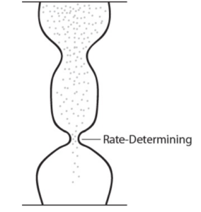
Image from Introduction to Chemistry, 1st Canadian Edition / CC BY 4.0

Pre-Equilibria

Say we have the following forward and reverse reaction:

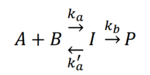
Consider a case where an equilibrium is established due to \(k_{a}’ >> k_{b}\):

The equilibrium constant, expressed using the forward and reverse reaction constants (\(k_{a}\) and \(k_{a}’\)) would remain the same over time

The reaction of \(I→P\) would decrease \([I]\) over time. Due to Le Chatelier’s principle, the equilibrium reaction will shift to produce more \(I\)

Because \(k_{a}'>>k_{b}\), the reaction will shift concentrations to achieve equilibrium again far faster than the forward reaction (\(k_{b}\)) depletes \(I\)

Therefore, we can approximate \([I]\) with only the equilibrium part of the reaction

\(K=\Big(\frac{[I]}{[A][B]}\Big)_{eq}c^\theta=\frac{k_{a}}{k'_{a}}c^\theta\)

Review: From lecture 4: reaction equilibrium:

The forward reaction: \(A+B\xrightarrow{\text{ka}}I\), reaction rate \(r=k_{a}[A][B]\)

The reverse reaction: \(I\xrightarrow{\text{k'a}}A+B\), reaction rate \(r'=k_{a}'[I]\)

At equilibrium: \begin{align*}
r & =r’\\
k_{a}[A][B] & = k_{a}'[I]\\
\frac{k_{a}}{k_{a}’}& = \frac{[I]}{[A][B]}
\end{align*}

So

\([I]=\frac{K}{c^\theta}[A][B]=\frac{k_{a}}{k_{a}'}[A][B]\)

Using the equation for \([I]\) based on this equilibrium, we can develop an equation for the rate of formation of \(P\):

\(\frac{d[P]}{dt}=k_{b}[I]=k_{b}\frac{k_{a}}{k_{a}'}[A][B]=k_{r}[A][B]\)

Where \(k_{r}=k_{b}\frac{k_{a}}{k_{a}'}\). The final step of \(I→P\) is rate determining, whereas the steps prior control the amount of intermediate.

Relate \(k_{r}\) to Activation Energy

Recall from Lecture 4:

For each step of the reaction, we can use the Arrhenius equation to substitute \(k_{r}=Ae^{(-\frac{E_{a}}{RT})}\), where \(A\) is the frequency factor and \(E_{a}\) is the activation energy

So we can express the overall rate constant of the reaction above as:

\[k_{r}=\frac{A_{a}e^{-\frac{Ea,a}{RT}}A_{b}e^{-\frac{Ea,b}{RT}}}{A_{a}'e^{-\frac{Ea,a'}{RT}}}=\frac{A_{a}A_{b}}{A_{a}'}e^{-\frac{(Ea,a+Ea,b-Ea,a')}{RT}}\]

Although each rate constant may increase with temperature, this may not be true of the overall rate constant \(k_{r}\).

The effective activation energy is: \(E_{a}=E_{a}+E_{b}-E_{a}'\) and this may be positive or negative depending on \(E_{a}\) of individual steps.

Exercise: Using Pre-Equilibria to Find the Rate Law Expression

The two-step mechanism below has been proposed for a reaction between nitrogen monoxide and molecular chlorine:

Use this mechanism to derive the equation and predicted rate law for the overall reaction.

The rate law should be expressed in terms of \([NO]\), \([Cl_{2}]\), and the rate constants of the elementary reactions shown above.\(^{[3]}\)

Solution

Add example text here.

Step 1: The overall reaction is the sum of the 2 elementary reactions:

\[2NO_{(g)}+Cl_{2(g)}→2NOCl_{(g)}\]

Step 2: Write each reaction separately and express the rate law for each reaction (including the reverse reaction in the equilibrium):

\begin{align*}
NO_{(g)}+Cl_{2(g)}→NOCl_{2(g)},\;\;\; & r_{1}=k_{a}[NO][Cl_{2}]\\
NOCl_{2(g)}→NO_{(g)}+Cl_{2(g)},\;\;\; & r_{-1}=k_{a}'[NOCl_{2}]\\
NOCl_{2}+NO→2NOCl,\;\;\; & r_{2}=k_{b}[NOCl_{2}][NO]
\end{align*}

Step 3: Use the equilibrium reaction to express the concentration of the intermediate (\([NOCl_{2}]\)):

\[[NOCl_{2}]=\frac{k_{a}}{k_{a}'}[NO][Cl_{2}]\]

Step 4: Express the overall reaction rate using the step 2 elementary reaction, then subsitute in \([NOCl_{2}]\):
\begin{align*}
overall\;rate&=\frac{1}{2}\frac{d[NOCl]}{dt}\\
&=\frac{2k_{b}[NO][NOCl_{2}]}{2}\\
&=k_{b}[NO][NOCl_{2}]\\
&=\frac{k_{b}k_{a}}{k_{a}’}[NO]^2[Cl_{2}]
\end{align*}

References

[1] Chemistry LibreTexts. 2020. Steady State Approximation. [online] Available at: <https://chem.libretexts.org/Bookshelves/Physical_and_Theoretical_Chemistry_Textbook_Maps/Supplemental_Modules_(Physical_and_Theoretical_Chemistry)/Kinetics/Reaction_Mechanisms/Steady-State_Approximation> [Accessed 04 May, 2020].

[2] Introduction to Chemistry. 1st Canadian Edition. 2014. Reaction Mechanisms. [online] Available at: <https://opentextbc.ca/introductorychemistry/chapter/reaction-mechanisms-2/> [Accessed 04 May, 2020].

[3] OpenStax Chemistry 2e. 2019. 12.6 Reaction Mechanisms. [online] Available at: <https://openstax.org/books/chemistry-2e/pages/12-6-reaction-mechanisms> [Accessed 05 May, 2020].