5.2: The Streamfunction
- Page ID
- 18064
\( \newcommand{\vecs}[1]{\overset { \scriptstyle \rightharpoonup} {\mathbf{#1}} } \)
\( \newcommand{\vecd}[1]{\overset{-\!-\!\rightharpoonup}{\vphantom{a}\smash {#1}}} \)
\( \newcommand{\id}{\mathrm{id}}\) \( \newcommand{\Span}{\mathrm{span}}\)
( \newcommand{\kernel}{\mathrm{null}\,}\) \( \newcommand{\range}{\mathrm{range}\,}\)
\( \newcommand{\RealPart}{\mathrm{Re}}\) \( \newcommand{\ImaginaryPart}{\mathrm{Im}}\)
\( \newcommand{\Argument}{\mathrm{Arg}}\) \( \newcommand{\norm}[1]{\| #1 \|}\)
\( \newcommand{\inner}[2]{\langle #1, #2 \rangle}\)
\( \newcommand{\Span}{\mathrm{span}}\)
\( \newcommand{\id}{\mathrm{id}}\)
\( \newcommand{\Span}{\mathrm{span}}\)
\( \newcommand{\kernel}{\mathrm{null}\,}\)
\( \newcommand{\range}{\mathrm{range}\,}\)
\( \newcommand{\RealPart}{\mathrm{Re}}\)
\( \newcommand{\ImaginaryPart}{\mathrm{Im}}\)
\( \newcommand{\Argument}{\mathrm{Arg}}\)
\( \newcommand{\norm}[1]{\| #1 \|}\)
\( \newcommand{\inner}[2]{\langle #1, #2 \rangle}\)
\( \newcommand{\Span}{\mathrm{span}}\) \( \newcommand{\AA}{\unicode[.8,0]{x212B}}\)
\( \newcommand{\vectorA}[1]{\vec{#1}} % arrow\)
\( \newcommand{\vectorAt}[1]{\vec{\text{#1}}} % arrow\)
\( \newcommand{\vectorB}[1]{\overset { \scriptstyle \rightharpoonup} {\mathbf{#1}} } \)
\( \newcommand{\vectorC}[1]{\textbf{#1}} \)
\( \newcommand{\vectorD}[1]{\overrightarrow{#1}} \)
\( \newcommand{\vectorDt}[1]{\overrightarrow{\text{#1}}} \)
\( \newcommand{\vectE}[1]{\overset{-\!-\!\rightharpoonup}{\vphantom{a}\smash{\mathbf {#1}}}} \)
\( \newcommand{\vecs}[1]{\overset { \scriptstyle \rightharpoonup} {\mathbf{#1}} } \)
\( \newcommand{\vecd}[1]{\overset{-\!-\!\rightharpoonup}{\vphantom{a}\smash {#1}}} \)
\(\newcommand{\avec}{\mathbf a}\) \(\newcommand{\bvec}{\mathbf b}\) \(\newcommand{\cvec}{\mathbf c}\) \(\newcommand{\dvec}{\mathbf d}\) \(\newcommand{\dtil}{\widetilde{\mathbf d}}\) \(\newcommand{\evec}{\mathbf e}\) \(\newcommand{\fvec}{\mathbf f}\) \(\newcommand{\nvec}{\mathbf n}\) \(\newcommand{\pvec}{\mathbf p}\) \(\newcommand{\qvec}{\mathbf q}\) \(\newcommand{\svec}{\mathbf s}\) \(\newcommand{\tvec}{\mathbf t}\) \(\newcommand{\uvec}{\mathbf u}\) \(\newcommand{\vvec}{\mathbf v}\) \(\newcommand{\wvec}{\mathbf w}\) \(\newcommand{\xvec}{\mathbf x}\) \(\newcommand{\yvec}{\mathbf y}\) \(\newcommand{\zvec}{\mathbf z}\) \(\newcommand{\rvec}{\mathbf r}\) \(\newcommand{\mvec}{\mathbf m}\) \(\newcommand{\zerovec}{\mathbf 0}\) \(\newcommand{\onevec}{\mathbf 1}\) \(\newcommand{\real}{\mathbb R}\) \(\newcommand{\twovec}[2]{\left[\begin{array}{r}#1 \\ #2 \end{array}\right]}\) \(\newcommand{\ctwovec}[2]{\left[\begin{array}{c}#1 \\ #2 \end{array}\right]}\) \(\newcommand{\threevec}[3]{\left[\begin{array}{r}#1 \\ #2 \\ #3 \end{array}\right]}\) \(\newcommand{\cthreevec}[3]{\left[\begin{array}{c}#1 \\ #2 \\ #3 \end{array}\right]}\) \(\newcommand{\fourvec}[4]{\left[\begin{array}{r}#1 \\ #2 \\ #3 \\ #4 \end{array}\right]}\) \(\newcommand{\cfourvec}[4]{\left[\begin{array}{c}#1 \\ #2 \\ #3 \\ #4 \end{array}\right]}\) \(\newcommand{\fivevec}[5]{\left[\begin{array}{r}#1 \\ #2 \\ #3 \\ #4 \\ #5 \\ \end{array}\right]}\) \(\newcommand{\cfivevec}[5]{\left[\begin{array}{c}#1 \\ #2 \\ #3 \\ #4 \\ #5 \\ \end{array}\right]}\) \(\newcommand{\mattwo}[4]{\left[\begin{array}{rr}#1 \amp #2 \\ #3 \amp #4 \\ \end{array}\right]}\) \(\newcommand{\laspan}[1]{\text{Span}\{#1\}}\) \(\newcommand{\bcal}{\cal B}\) \(\newcommand{\ccal}{\cal C}\) \(\newcommand{\scal}{\cal S}\) \(\newcommand{\wcal}{\cal W}\) \(\newcommand{\ecal}{\cal E}\) \(\newcommand{\coords}[2]{\left\{#1\right\}_{#2}}\) \(\newcommand{\gray}[1]{\color{gray}{#1}}\) \(\newcommand{\lgray}[1]{\color{lightgray}{#1}}\) \(\newcommand{\rank}{\operatorname{rank}}\) \(\newcommand{\row}{\text{Row}}\) \(\newcommand{\col}{\text{Col}}\) \(\renewcommand{\row}{\text{Row}}\) \(\newcommand{\nul}{\text{Nul}}\) \(\newcommand{\var}{\text{Var}}\) \(\newcommand{\corr}{\text{corr}}\) \(\newcommand{\len}[1]{\left|#1\right|}\) \(\newcommand{\bbar}{\overline{\bvec}}\) \(\newcommand{\bhat}{\widehat{\bvec}}\) \(\newcommand{\bperp}{\bvec^\perp}\) \(\newcommand{\xhat}{\widehat{\xvec}}\) \(\newcommand{\vhat}{\widehat{\vvec}}\) \(\newcommand{\uhat}{\widehat{\uvec}}\) \(\newcommand{\what}{\widehat{\wvec}}\) \(\newcommand{\Sighat}{\widehat{\Sigma}}\) \(\newcommand{\lt}{<}\) \(\newcommand{\gt}{>}\) \(\newcommand{\amp}{&}\) \(\definecolor{fillinmathshade}{gray}{0.9}\)
Many flows are approximately two-dimensional. For example, the thickness of the Earth’s atmosphere relative to the planet is comparable to the skin on an apple. Large-scale atmospheric flows are therefore nearly two-dimensional. When a flow is two-dimensional and also incompressible \( \left( \vec{\nabla}\cdot\vec{u}=0 \right) \), it can represented by means of a streamfunction \(\psi\). Suppose the two dimensions are \(x\) and \(y\), with corresponding velocity components \(u(x, y)\) and \(v(x, y)\). Then \(\psi\) is defined such that
\[u=-\frac{\partial \Psi}{\partial y} ; \quad v=\frac{\partial \Psi}{\partial x} \label{eqn:1} \]
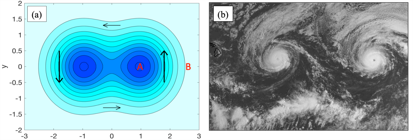
Curves of constant \(\psi\) are called streamlines. The simple example of a pair of nearby minima is shown in (Figure 5.2(a)).
Several properties of the streamfunction are noteworthy.
- The definition Equation \(\ref{eqn:1}\) guarantees that \(\vec{\nabla}\cdot\vec{u}\) will be zero. (Check this for yourself.)
- The sign convention is arbitrary. The present convention leads to \(\omega^{(z)} = +\nabla^2\psi\).
- You can add any fixed number to \(Ψ\) and it makes no difference to the resulting flow. In other words, the streamfunction is defined only up to an additive constant.
- The direction of the flow vector \(\vec{u}\) is perpendicular to \(\vec{\nabla}\psi\) or, equivalently, parallel to the streamlines: \[\vec{u} \cdot \vec{\nabla} \Psi=u \frac{\partial \Psi}{\partial x}+v \frac{\partial \Psi}{\partial y}=u v-v u=0, \nonumber \] using Equation \(\ref{eqn:1}\).
- The flow direction is defined more fully by noting the signs of the derivatives in Equation \(\ref{eqn:1}\). These require that flow be clockwise around a maximum in \(\psi\) and counterclockwise around a minimum (such as the pair of minima in Figure \(\PageIndex{1}\)). In (Figure \(\PageIndex{1}\)a), the streamfunction increases (becomes less negative) from point “A” to point “B”, hence \(\partial\psi/\partial x > 0\), hence \(v > 0\).
- The speed (velocity magnitude) is \(\sqrt{u^2+v^2} = |\vec{\nabla}\psi|\). Therefore, the flow is fastest where streamlines are clustered together, such as just outside the two peaks on (Figure \(\PageIndex{1}\)a). Flow is slow where streamlines are widely spaced.
Given the velocity components \(u\), \(v\), one can easily invert Equation \(\ref{eqn:1}\) to obtain the streamfunction. We can start with either equation; here we’ll pick the first one. Integrating:
\[\Psi=-\int u \, d y+f(x), \nonumber \]
where \(f\) is an unknown function independent of \(y\). Substituting this into the second of Equation \(\ref{eqn:1}\) gives
\[\frac{\partial \Psi}{\partial x}=-\int \frac{\partial u}{\partial x} d y+f^{\prime}(x)=v. \nonumber \]
This is readily solved for \(f^\prime\), which we integrate to obtain \(f\). Note that the constant of integration is arbitrary because of point 3 above.
Test your understanding by doing exercise 23, parts (a) and (b).