
1.6: Arches and Cables
- Page ID
- 17612

\( \newcommand{\vecs}[1]{\overset { \scriptstyle \rightharpoonup} {\mathbf{#1}} } \)
\( \newcommand{\vecd}[1]{\overset{-\!-\!\rightharpoonup}{\vphantom{a}\smash {#1}}} \)
\( \newcommand{\dsum}{\displaystyle\sum\limits} \)
\( \newcommand{\dint}{\displaystyle\int\limits} \)
\( \newcommand{\dlim}{\displaystyle\lim\limits} \)
\( \newcommand{\id}{\mathrm{id}}\) \( \newcommand{\Span}{\mathrm{span}}\)
( \newcommand{\kernel}{\mathrm{null}\,}\) \( \newcommand{\range}{\mathrm{range}\,}\)
\( \newcommand{\RealPart}{\mathrm{Re}}\) \( \newcommand{\ImaginaryPart}{\mathrm{Im}}\)
\( \newcommand{\Argument}{\mathrm{Arg}}\) \( \newcommand{\norm}[1]{\| #1 \|}\)
\( \newcommand{\inner}[2]{\langle #1, #2 \rangle}\)
\( \newcommand{\Span}{\mathrm{span}}\)
\( \newcommand{\id}{\mathrm{id}}\)
\( \newcommand{\Span}{\mathrm{span}}\)
\( \newcommand{\kernel}{\mathrm{null}\,}\)
\( \newcommand{\range}{\mathrm{range}\,}\)
\( \newcommand{\RealPart}{\mathrm{Re}}\)
\( \newcommand{\ImaginaryPart}{\mathrm{Im}}\)
\( \newcommand{\Argument}{\mathrm{Arg}}\)
\( \newcommand{\norm}[1]{\| #1 \|}\)
\( \newcommand{\inner}[2]{\langle #1, #2 \rangle}\)
\( \newcommand{\Span}{\mathrm{span}}\) \( \newcommand{\AA}{\unicode[.8,0]{x212B}}\)
\( \newcommand{\vectorA}[1]{\vec{#1}} % arrow\)
\( \newcommand{\vectorAt}[1]{\vec{\text{#1}}} % arrow\)
\( \newcommand{\vectorB}[1]{\overset { \scriptstyle \rightharpoonup} {\mathbf{#1}} } \)
\( \newcommand{\vectorC}[1]{\textbf{#1}} \)
\( \newcommand{\vectorD}[1]{\overrightarrow{#1}} \)
\( \newcommand{\vectorDt}[1]{\overrightarrow{\text{#1}}} \)
\( \newcommand{\vectE}[1]{\overset{-\!-\!\rightharpoonup}{\vphantom{a}\smash{\mathbf {#1}}}} \)
\( \newcommand{\vecs}[1]{\overset { \scriptstyle \rightharpoonup} {\mathbf{#1}} } \)
\(\newcommand{\longvect}{\overrightarrow}\)
\( \newcommand{\vecd}[1]{\overset{-\!-\!\rightharpoonup}{\vphantom{a}\smash {#1}}} \)
\(\newcommand{\avec}{\mathbf a}\) \(\newcommand{\bvec}{\mathbf b}\) \(\newcommand{\cvec}{\mathbf c}\) \(\newcommand{\dvec}{\mathbf d}\) \(\newcommand{\dtil}{\widetilde{\mathbf d}}\) \(\newcommand{\evec}{\mathbf e}\) \(\newcommand{\fvec}{\mathbf f}\) \(\newcommand{\nvec}{\mathbf n}\) \(\newcommand{\pvec}{\mathbf p}\) \(\newcommand{\qvec}{\mathbf q}\) \(\newcommand{\svec}{\mathbf s}\) \(\newcommand{\tvec}{\mathbf t}\) \(\newcommand{\uvec}{\mathbf u}\) \(\newcommand{\vvec}{\mathbf v}\) \(\newcommand{\wvec}{\mathbf w}\) \(\newcommand{\xvec}{\mathbf x}\) \(\newcommand{\yvec}{\mathbf y}\) \(\newcommand{\zvec}{\mathbf z}\) \(\newcommand{\rvec}{\mathbf r}\) \(\newcommand{\mvec}{\mathbf m}\) \(\newcommand{\zerovec}{\mathbf 0}\) \(\newcommand{\onevec}{\mathbf 1}\) \(\newcommand{\real}{\mathbb R}\) \(\newcommand{\twovec}[2]{\left[\begin{array}{r}#1 \\ #2 \end{array}\right]}\) \(\newcommand{\ctwovec}[2]{\left[\begin{array}{c}#1 \\ #2 \end{array}\right]}\) \(\newcommand{\threevec}[3]{\left[\begin{array}{r}#1 \\ #2 \\ #3 \end{array}\right]}\) \(\newcommand{\cthreevec}[3]{\left[\begin{array}{c}#1 \\ #2 \\ #3 \end{array}\right]}\) \(\newcommand{\fourvec}[4]{\left[\begin{array}{r}#1 \\ #2 \\ #3 \\ #4 \end{array}\right]}\) \(\newcommand{\cfourvec}[4]{\left[\begin{array}{c}#1 \\ #2 \\ #3 \\ #4 \end{array}\right]}\) \(\newcommand{\fivevec}[5]{\left[\begin{array}{r}#1 \\ #2 \\ #3 \\ #4 \\ #5 \\ \end{array}\right]}\) \(\newcommand{\cfivevec}[5]{\left[\begin{array}{c}#1 \\ #2 \\ #3 \\ #4 \\ #5 \\ \end{array}\right]}\) \(\newcommand{\mattwo}[4]{\left[\begin{array}{rr}#1 \amp #2 \\ #3 \amp #4 \\ \end{array}\right]}\) \(\newcommand{\laspan}[1]{\text{Span}\{#1\}}\) \(\newcommand{\bcal}{\cal B}\) \(\newcommand{\ccal}{\cal C}\) \(\newcommand{\scal}{\cal S}\) \(\newcommand{\wcal}{\cal W}\) \(\newcommand{\ecal}{\cal E}\) \(\newcommand{\coords}[2]{\left\{#1\right\}_{#2}}\) \(\newcommand{\gray}[1]{\color{gray}{#1}}\) \(\newcommand{\lgray}[1]{\color{lightgray}{#1}}\) \(\newcommand{\rank}{\operatorname{rank}}\) \(\newcommand{\row}{\text{Row}}\) \(\newcommand{\col}{\text{Col}}\) \(\renewcommand{\row}{\text{Row}}\) \(\newcommand{\nul}{\text{Nul}}\) \(\newcommand{\var}{\text{Var}}\) \(\newcommand{\corr}{\text{corr}}\) \(\newcommand{\len}[1]{\left|#1\right|}\) \(\newcommand{\bbar}{\overline{\bvec}}\) \(\newcommand{\bhat}{\widehat{\bvec}}\) \(\newcommand{\bperp}{\bvec^\perp}\) \(\newcommand{\xhat}{\widehat{\xvec}}\) \(\newcommand{\vhat}{\widehat{\vvec}}\) \(\newcommand{\uhat}{\widehat{\uvec}}\) \(\newcommand{\what}{\widehat{\wvec}}\) \(\newcommand{\Sighat}{\widehat{\Sigma}}\) \(\newcommand{\lt}{<}\) \(\newcommand{\gt}{>}\) \(\newcommand{\amp}{&}\) \(\definecolor{fillinmathshade}{gray}{0.9}\)Arches are structures composed of curvilinear members resting on supports. They are used for large-span structures, such as airplane hangars and long-span bridges. One of the main distinguishing features of an arch is the development of horizontal thrusts at the supports as well as the vertical reactions, even in the absence of a horizontal load. The internal forces at any section of an arch include axial compression, shearing force, and bending moment. The bending moment and shearing force at such section of an arch are comparatively smaller than those of a beam of the same span due to the presence of the horizontal thrusts. The horizontal thrusts significantly reduce the moments and shear forces at any section of the arch, which results in reduced member size and a more economical design compared to other structures. Additionally, arches are also aesthetically more pleasant than most structures.
6.1.1 Types of Arches
Based on their geometry, arches can be classified as semicircular, segmental, or pointed. Based on the number of internal hinges, they can be further classified as two-hinged arches, three-hinged arches, or fixed arches, as seen in Figure 6.1. This chapter discusses the analysis of three-hinge arches only.
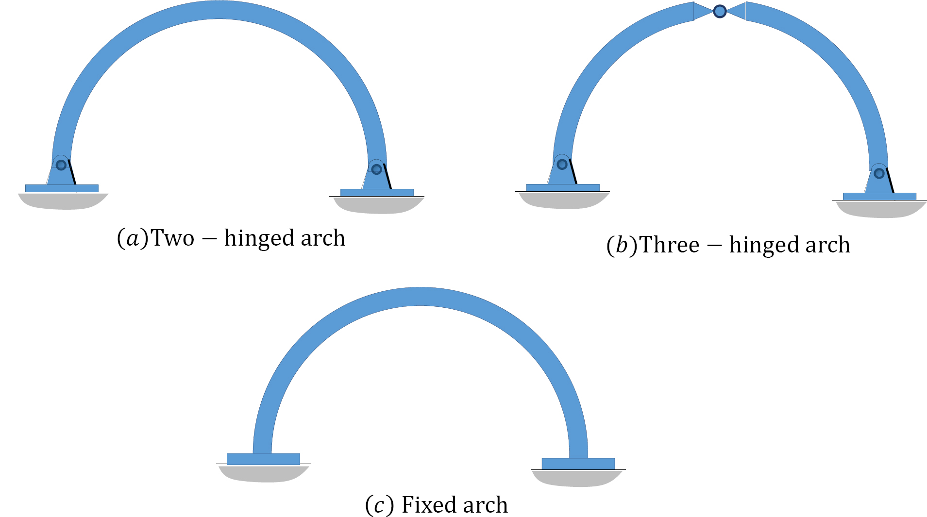
6.1.2 Three-Hinged Arch
A three-hinged arch is a geometrically stable and statically determinate structure. It consists of two curved members connected by an internal hinge at the crown and is supported by two hinges at its base. Sometimes, a tie is provided at the support level or at an elevated position in the arch to increase the stability of the structure.
6.1.2.1 Derivation of Equations for the Determination of Internal Forces in a Three-Hinged Arch
Consider the section Q in the three-hinged arch shown in Figure 6.2a. The three internal forces at the section are the axial force, NQ, the radial shear force, VQ, and the bending moment, MQ. The derivation of the equations for the determination of these forces with respect to the angle φ are as follows:
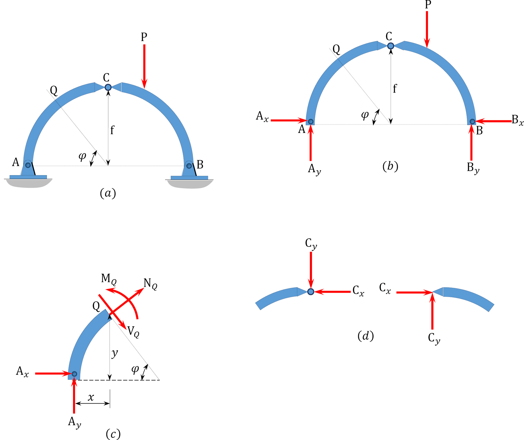
Bending moment at point Q.
\[M_{\varphi}=A_{y} x-A_{x} y=M_{(x)}^{b}-A_{x} y \label{6.1}\]
where
\(M_{(x)}^{b}\) = moment of a beam of the same span as the arch.
y = ordinate of any point along the central line of the arch.


f = rise of arch. This is the vertical distance from the centerline to the arch’s crown.
x = horizontal distance from the support to the section being considered.
L = span of arch.
R = radius of the arch’s curvature.
Radial shear force at point Q.
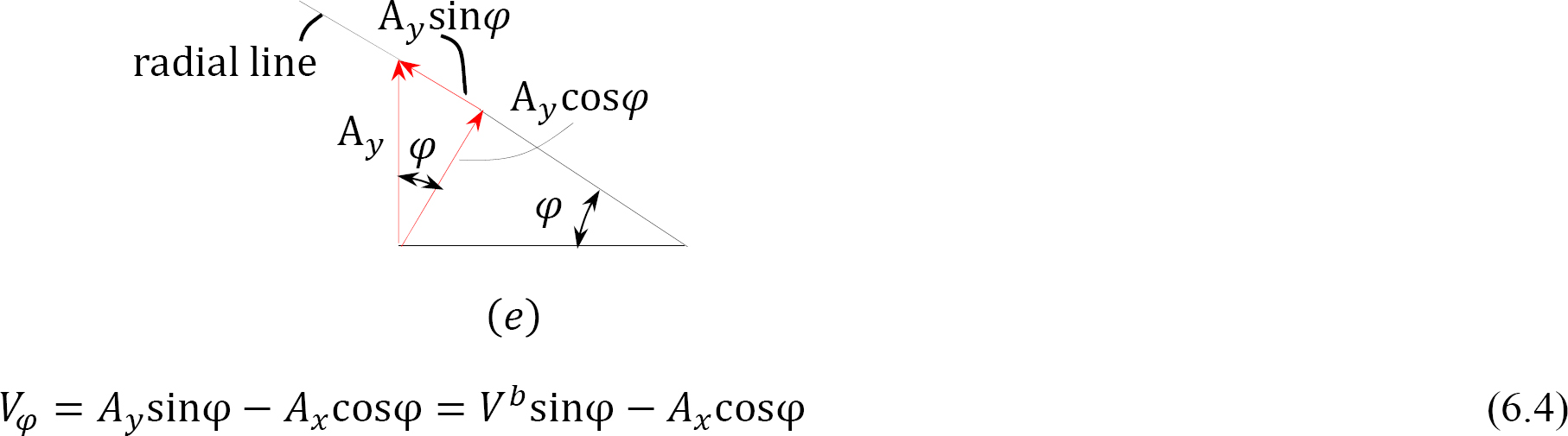
where
Vb = shear of a beam of the same span as the arch.
Axial force at a point Q.
\[N_{\varphi}=-A_{y} \cos \varphi-A_{x} \sin \varphi=-V^{b} \cos \varphi-A_{x} \sin \varphi \label{6.5}\]
A three-hinged arch is subjected to two concentrated loads, as shown in Figure 6.3a. Determine the support reactions of the arch.
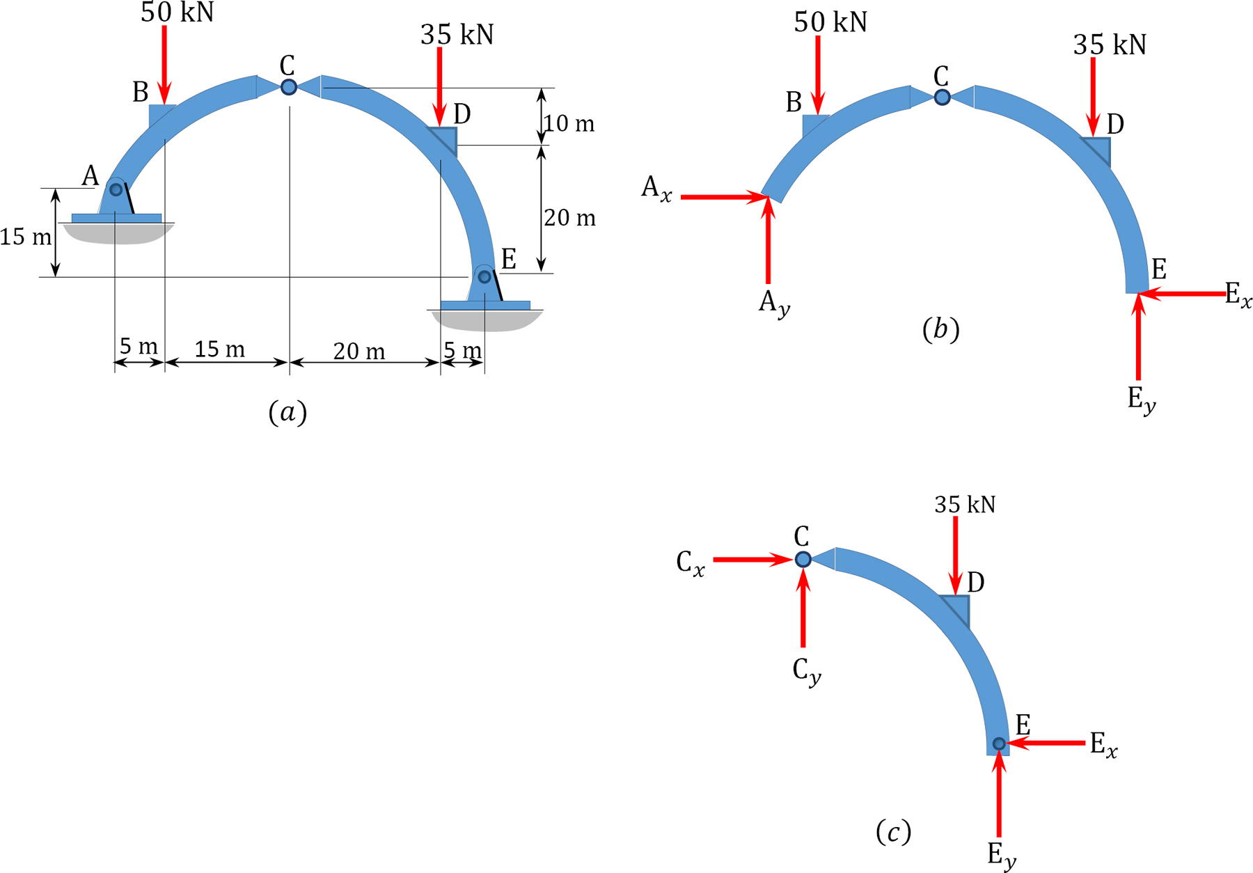
Solution
The free-body diagrams of the entire arch and its segment CE are shown in Figure 6.3b and Figure 6.3c, respectively. Applying the equations of static equilibrium suggests the following:
Entire arch.
Arch segment CE.
Solving equations 6.1 and 6.2 simultaneously yields the following:


Entire arch again.
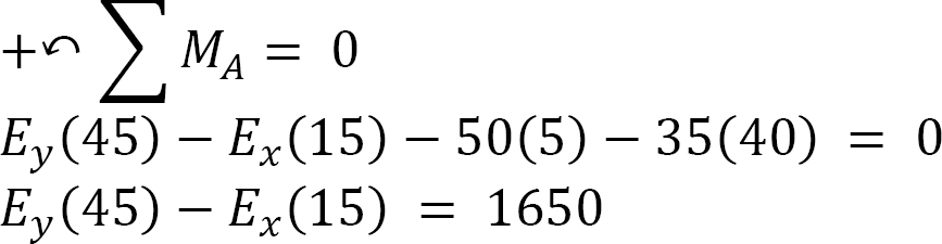
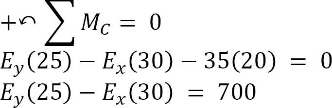
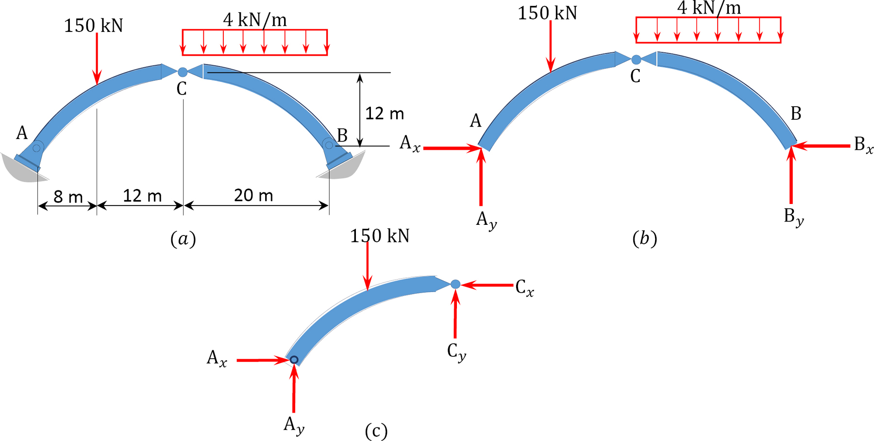
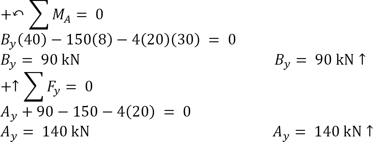
A parabolic arch with supports at the same level is subjected to the combined loading shown in Figure 6.4a. Determine the support reactions and the normal thrust and radial shear at a point just to the left of the 150 kN concentrated load.
Solution
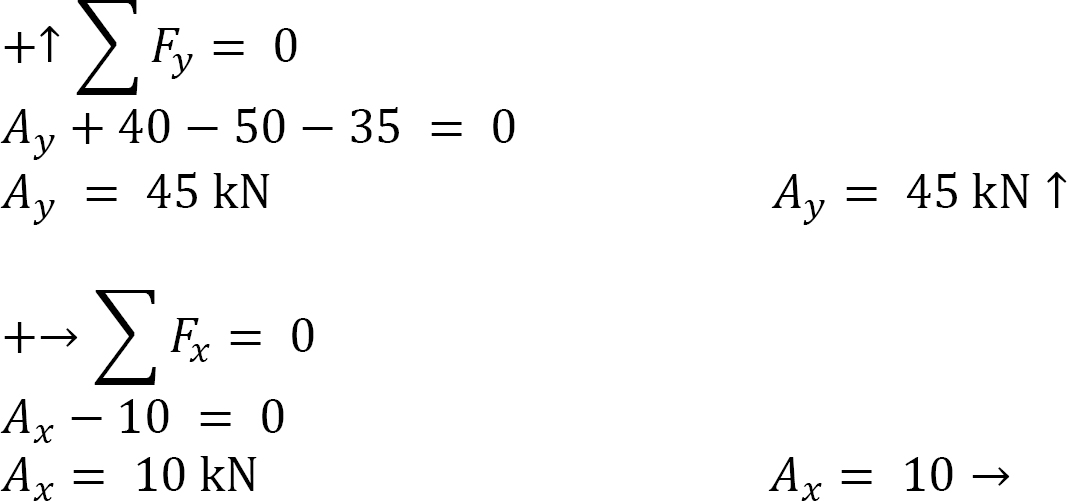
Support reactions. The free-body diagram of the entire arch is shown in Figure 6.4b, while that of its segment AC is shown in Figure 6.4c. Applying the equations of static equilibrium to determine the arch’s support reactions suggests the following:
Entire arch.
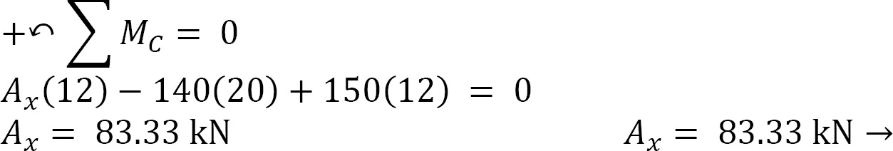
Arch segment AC.
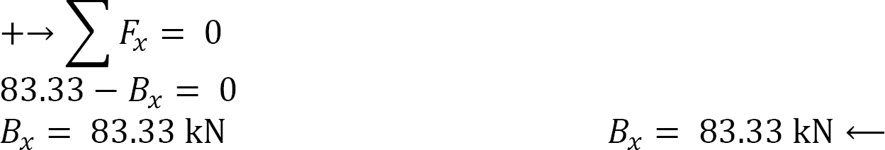
Entire arch again.
Normal thrust and radial shear. To determine the normal thrust and radial shear, find the angle between the horizontal and the arch just to the left of the 150 kN load.
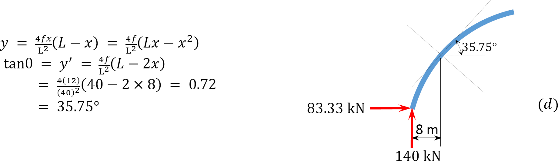
Normal thrust.

Radial shear.

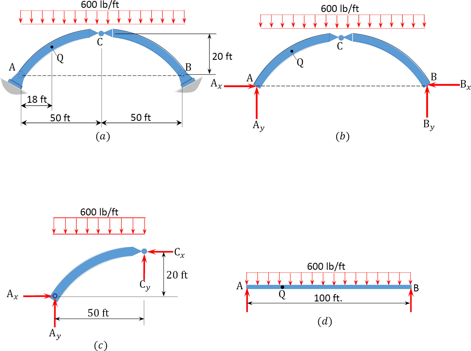
A parabolic arch is subjected to a uniformly distributed load of 600 lb/ft throughout its span, as shown in Figure 6.5a. Determine the support reactions and the bending moment at a section Q in the arch, which is at a distance of 18 ft from the left-hand support.
Solution
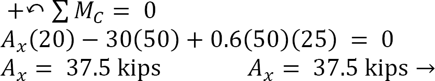
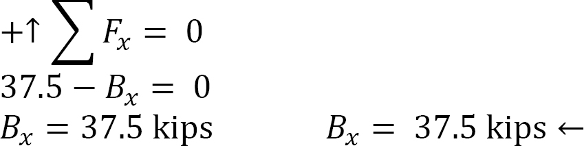
Support reactions. The free-body diagram of the entire arch is shown in Figure 6.5b, while that of its segment AC is shown Figure 6.5c. Applying the equations of static equilibrium for the determination of the arch’s support reactions suggests the following:
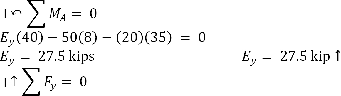
Free-body diagram of entire arch. Due to symmetry in loading, the vertical reactions in both supports of the arch are the same. Therefore,
\[A_{y}=B_{y}=\frac{w L}{2}=\frac{0.6(100)}{2}=30 \text { kips } \nonumber\]
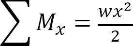
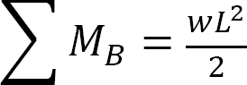
The horizontal thrust at both supports of the arch are the same, and they can be computed by considering the free body diagram in Figure 6.5b. Taking the moment about point C of the free-body diagram suggests the following:
Free-body diagram of segment AC. The horizontal thrust at both supports of the arch are the same, and they can be computed by considering the free body diagram in Figure 6.5c. Taking the moment about point C of the free-body diagram suggests the following:
Free-body diagram of entire arch again.
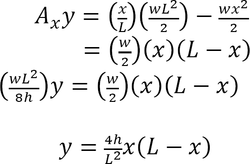
Bending moment at point Q: To find the bending moment at a point Q, which is located 18 ft from support A, first determine the ordinate of the arch at that point by using the equation of the ordinate of a parabola.
\[y=\frac{4 f x}{\mathrm{~L}^{2}}(L-x)\]
\[y_{x=18 \mathrm{ft}}=\frac{4(20)(18)}{(100)^{2}}(100-18)=11.81 \mathrm{ft}\]
The moment at Q can be determined as the summation of the moment of the forces on the left-hand portion of the point in the beam, as shown in Figure 6.5c, and the moment due to the horizontal thrust, Ax. Thus, MQ = Ay(18) – 0.6(18)(9) – Ax(11.81)

Example 6.4
A parabolic arch is subjected to two concentrated loads, as shown in Figure 6.6a. Determine the support reactions and draw the bending moment diagram for the arch.

Solution
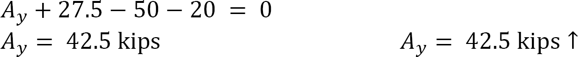
Support reactions. The free-body diagram of the entire arch is shown in Figure 6.6b. Applying the equations of static equilibrium determines the components of the support reactions and suggests the following:
Entire arch.
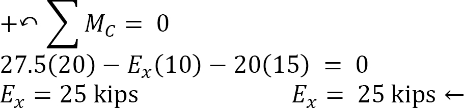
Arch segment EC.
For the horizontal reactions, sum the moments about the hinge at C.
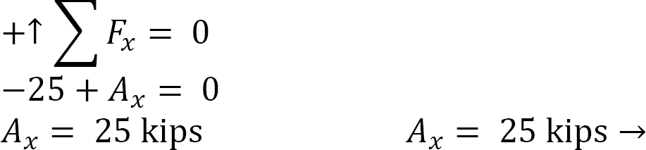
Entire arch again.
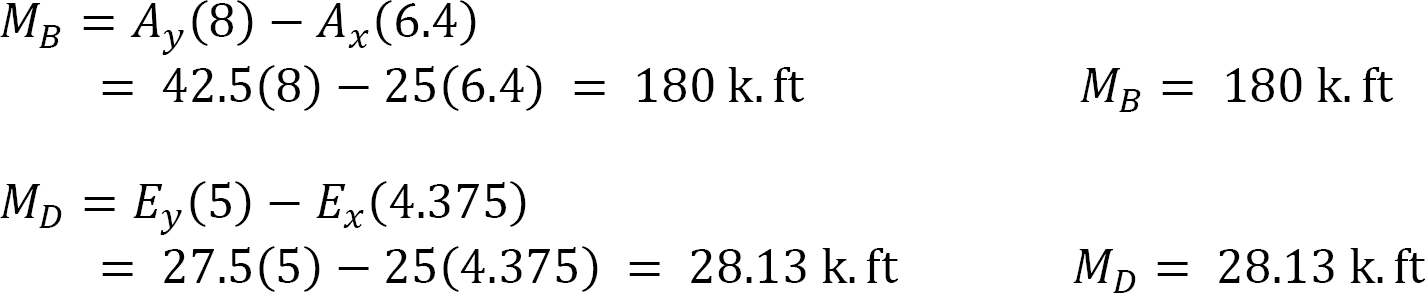
Bending moment at the locations of concentrated loads. To find the bending moments at sections of the arch subjected to concentrated loads, first determine the ordinates at these sections using the equation of the ordinate of a parabola, which is as follows:

Cables are flexible structures that support the applied transverse loads by the tensile resistance developed in its members. Cables are used in suspension bridges, tension leg offshore platforms, transmission lines, and several other engineering applications. The distinguishing feature of a cable is its ability to take different shapes when subjected to different types of loadings. Under a uniform load, a cable takes the shape of a curve, while under a concentrated load, it takes the form of several linear segments between the load’s points of application.
6.2.1 General Cable Theorem
The general cable theorem states that at any point on a cable that is supported at two ends and subjected to vertical transverse loads, the product of the horizontal component of the cable tension and the vertical distance from that point to the cable chord equals the moment which would occur at that section if the load carried by the cable were acting on a simply supported beam of the same span as that of the cable.
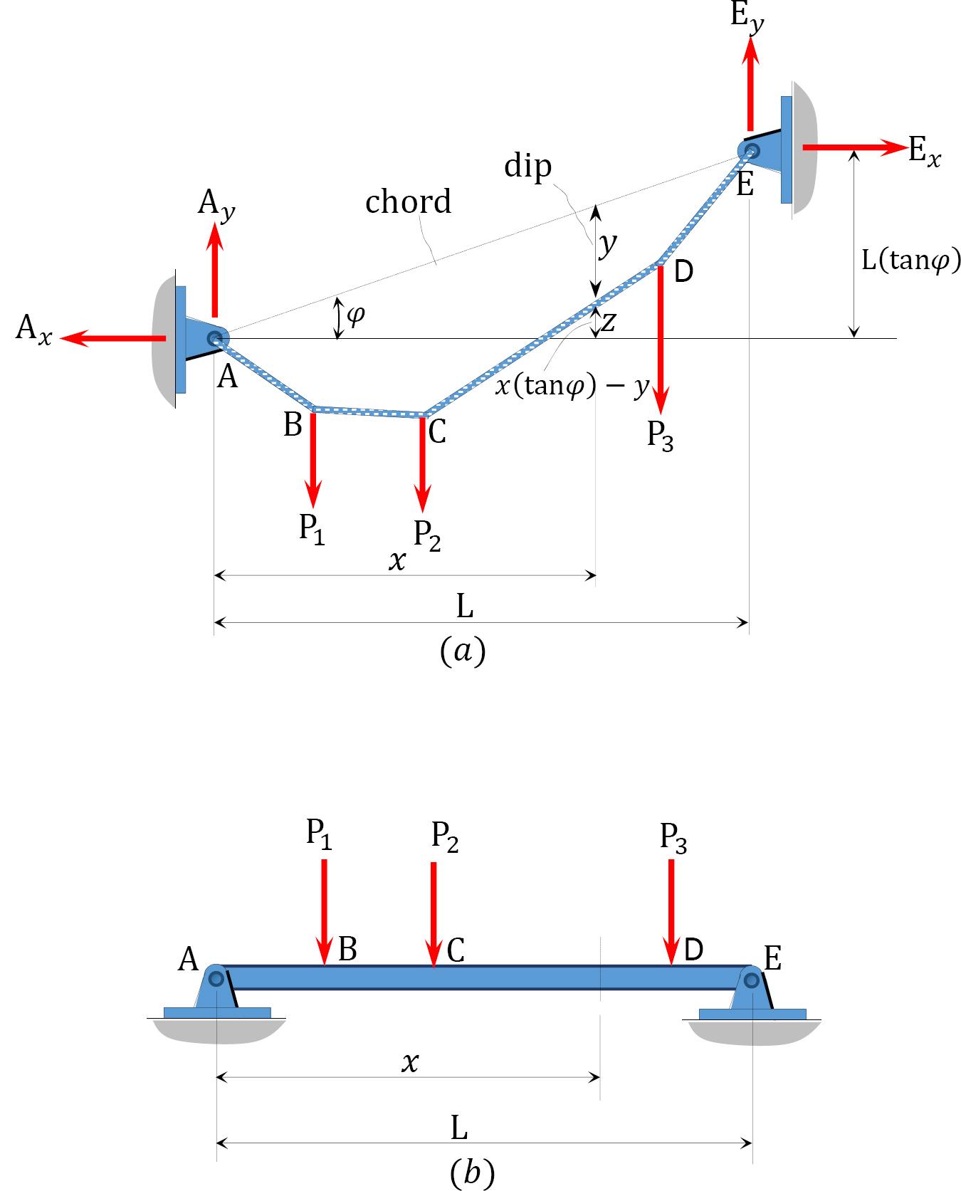
To prove the general cable theorem, consider the cable and the beam shown in Figure 6.7a and Figure 6.7b, respectively. Both structures are supported at both ends, have a span L, and are subjected to the same concentrated loads at B, C, and D. A line joining supports A and E is referred to as the chord, while a vertical height from the chord to the surface of the cable at any point of a distance x from the left support, as shown in Figure 6.7a, is known as the dip at that point. For equilibrium of a structure, the horizontal reactions at both supports must be the same. From static equilibrium, the moment of the forces on the cable about support B and about the section at a distance x from the left support can be expressed as follows, respectively:

where
∑ MBP = the algebraic sum of the moment of the applied forces about support B.


Substituting Ay from equation 6.8 into equation 6.7 suggests the following: 


Substituting Ay from equation 6.10 into equation 6.11 suggests the following:

The moment at a section of a beam at a distance x from the left support presented in equation 6.12 is the same as equation 6.9. This confirms the general cable theorem.
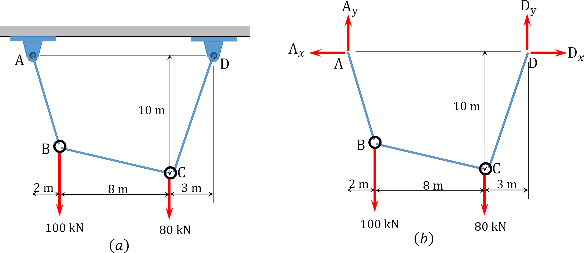
A cable supports two concentrated loads at B and C, as shown in Figure 6.8a. Determine the sag at B, the tension in the cable, and the length of the cable.
Solution
Support reactions. The reactions of the cable are determined by applying the equations of equilibrium to the free-body diagram of the cable shown in Figure 6.8b, which is written as follows:
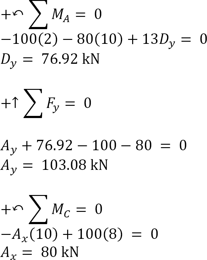
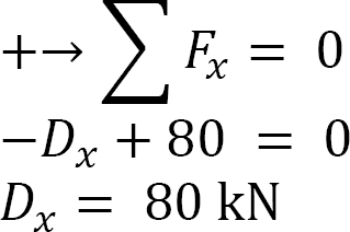
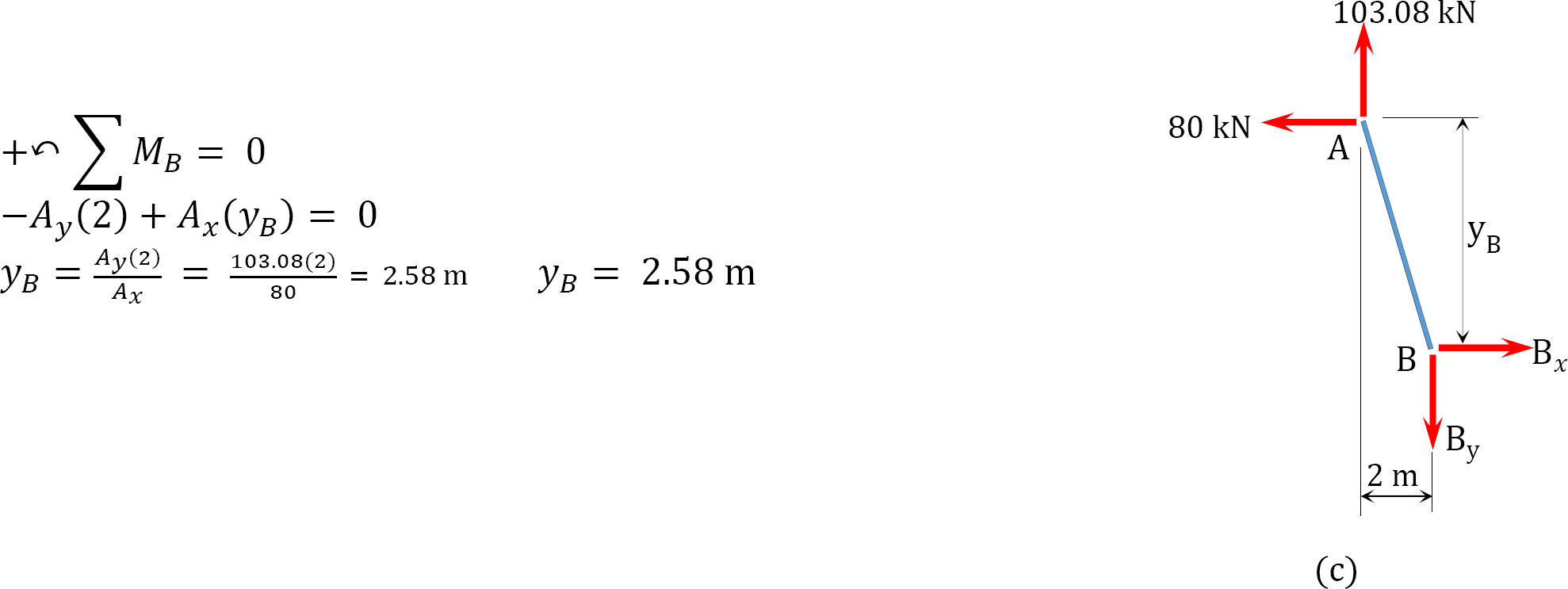
Tension in cable.
Tension at A and D.
Tension in segment CB.
Length of cable. The length of the cable is determined as the algebraic sum of the lengths of the segments. The lengths of the segments can be obtained by the application of the Pythagoras theorem, as follows:
\[L=\sqrt{(2.58)^{2}+(2)^{2}}+\sqrt{(10-2.58)^{2}+(8)^{2}}+\sqrt{(10)^{2}+(3)^{2}}=24.62 \mathrm{~m} \nonumber\]
Example 6.6
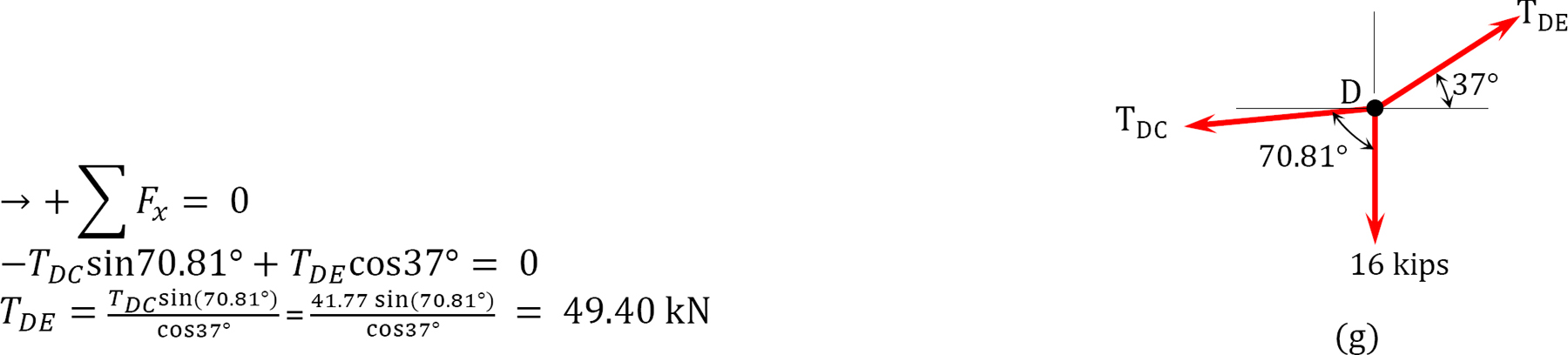
A cable supports three concentrated loads at B, C, and D, as shown in Figure 6.9a. Determine the sag at B and D, as well as the tension in each segment of the cable.

Solution
Support reactions. The reactions shown in the free-body diagram of the cable in Figure 6.9b are determined by applying the equations of equilibrium, which are written as follows:
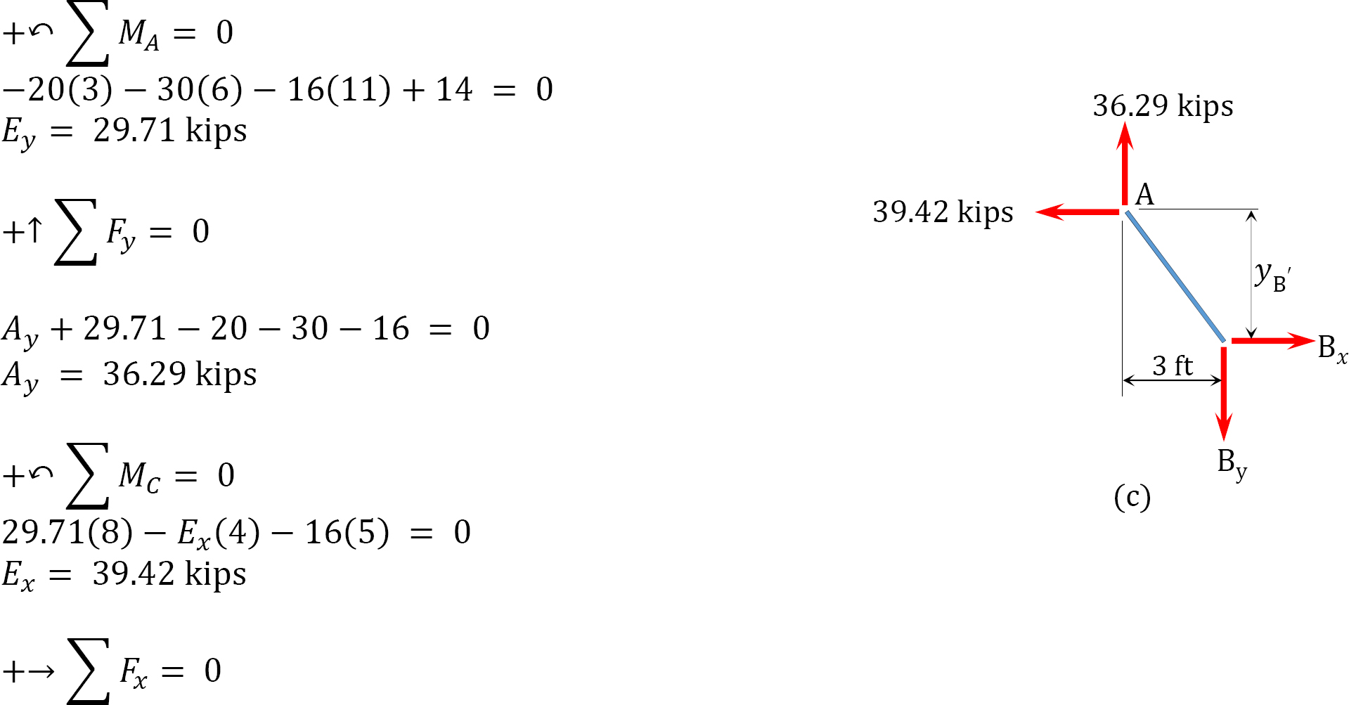
–Ax + 39.42 = 0
Ax = 39.42 kips
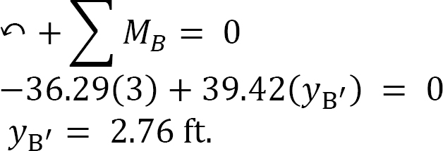
Sag. The sag at B is determined by summing the moment about B, as shown in the free-body diagram in Figure 6.9c, while the sag at D was computed by summing the moment about D, as shown in the free-body diagram in Figure 6.9d.
Sag at B.
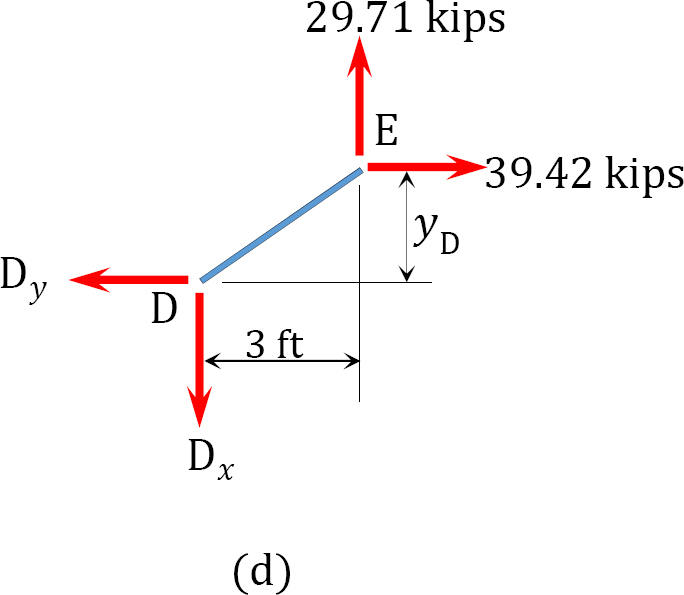
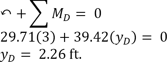
Sag at D.
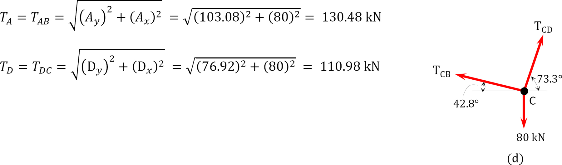
Tension.
Tension at A.

Tension at E.

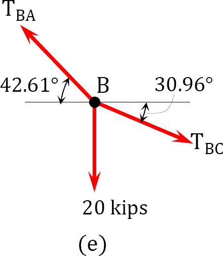
Tension at B.
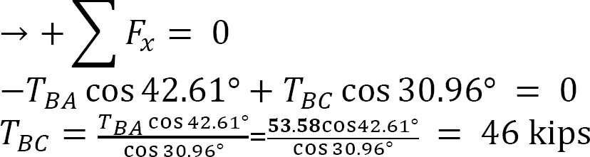
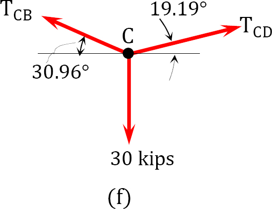
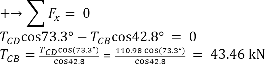
Tension at C.
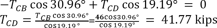
Tension at D.
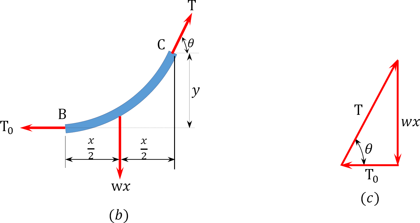
6.2.2 Parabolic Cable Carrying Horizontal Distributed Loads
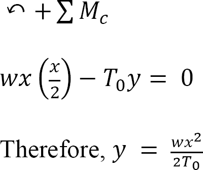
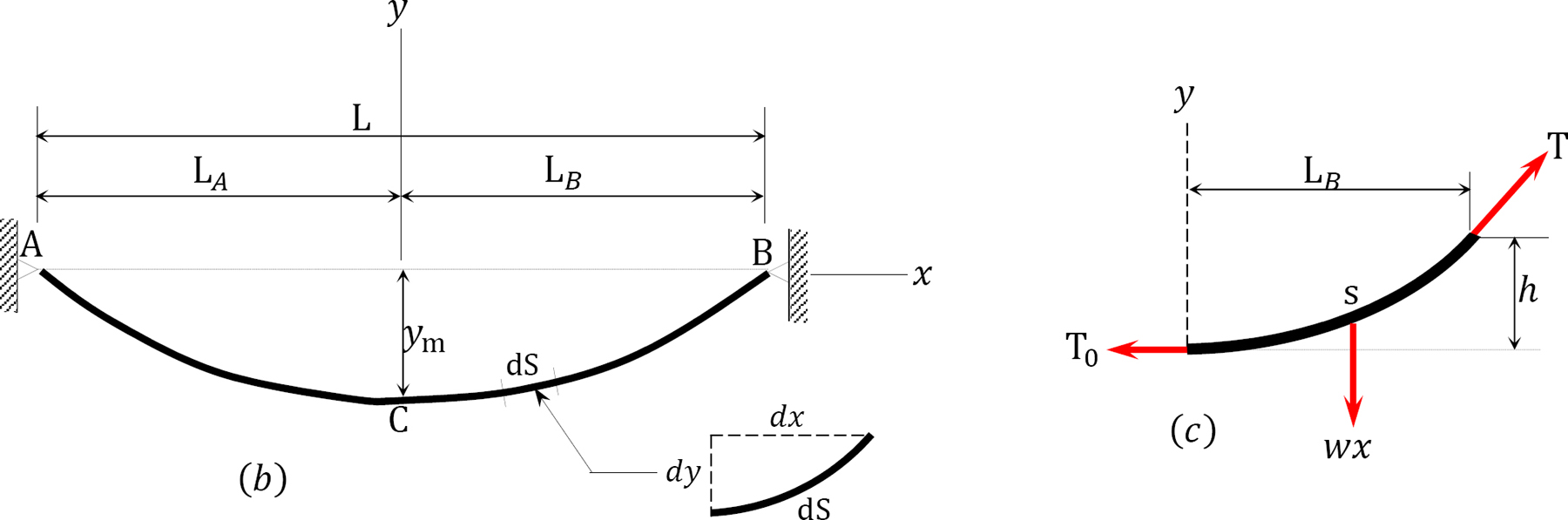
To develop the basic relationships for the analysis of parabolic cables, consider segment BC of the cable suspended from two points A and D, as shown in Figure 6.10a. Point B is the lowest point of the cable, while point C is an arbitrary point lying on the cable. Taking B as the origin and denoting the tensile horizontal force at this origin as T0 and denoting the tensile inclined force at C as T, as shown in Figure 6.10b, suggests the following:

Figure 6.10c suggests the following:

Equation 6.13 defines the slope of the curve of the cable with respect to x. To determine the vertical distance between the lowest point of the cable (point B) and the arbitrary point C, rearrange and further integrate equation 6.13, as follows:
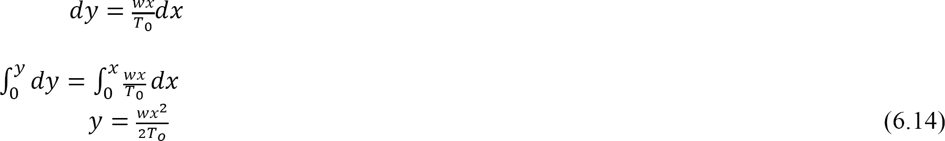

where
T and T0 are the maximum and minimum tensions in the cable, respectively.
Example 6.7
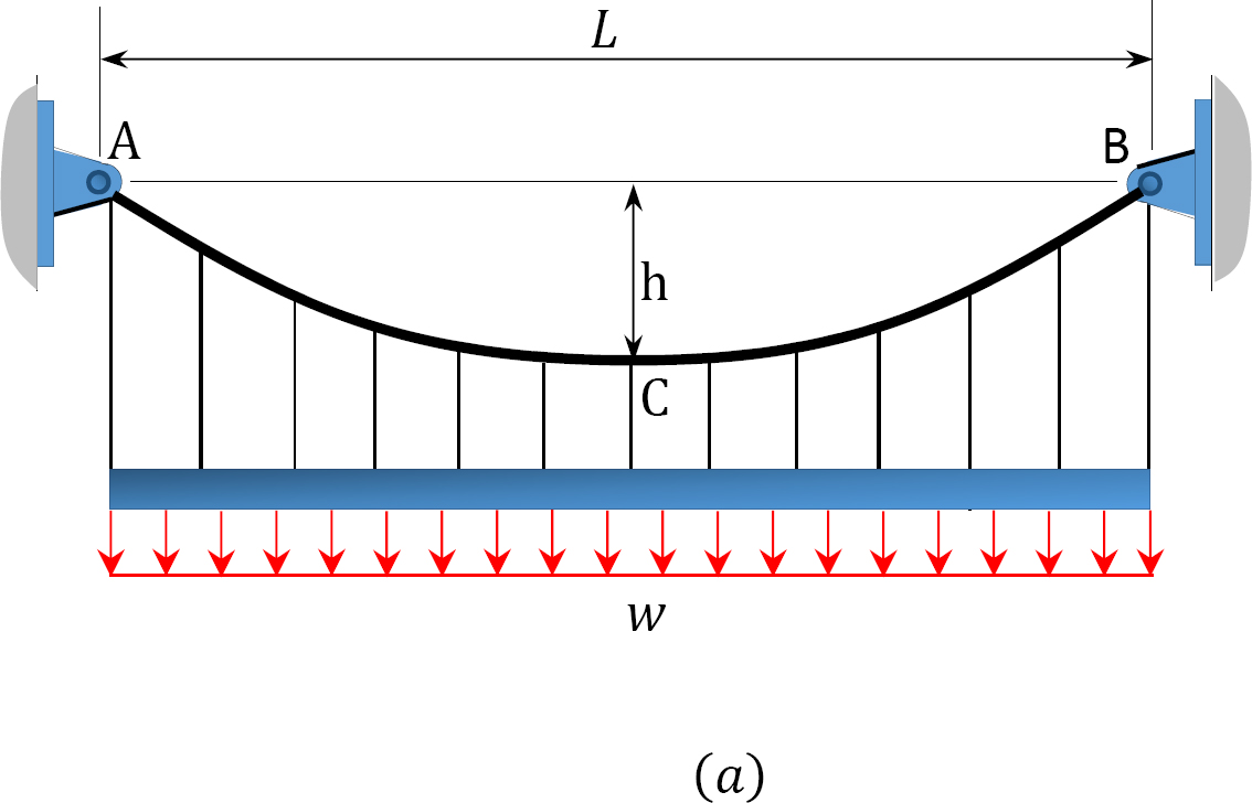
A cable supports a uniformly distributed load, as shown Figure 6.11a. Determine the horizontal reaction at the supports of the cable, the expression of the shape of the cable, and the length of the cable.
Solution
As the dip of the cable is known, apply the general cable theorem to find the horizontal reaction.
The expression of the shape of the cable is found using the following equations:
For any point P(x, y) on the cable, apply cable equation.
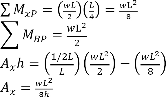
The moment at any section x due to the applied load is expressed as follows:
The moment at support B is written as follows:
Applying the general cable theorem yields the following:
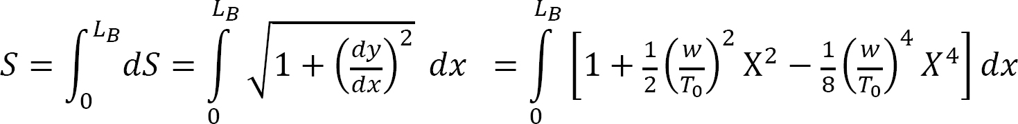
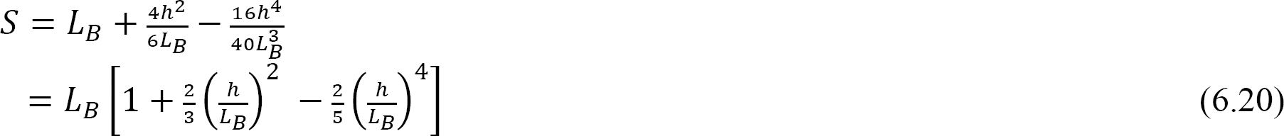
The length of the cable can be found using the following:
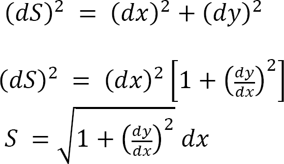

The solution of equation 6.16 can be simplified by expressing the radical under the integral as a series using a binomial expansion, as presented in equation 6.17, and then integrating each term.

Putting 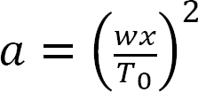 into three terms of the expansion in equation 6.13 suggests the following:

Thus, equation 6.16 can be written as the following:
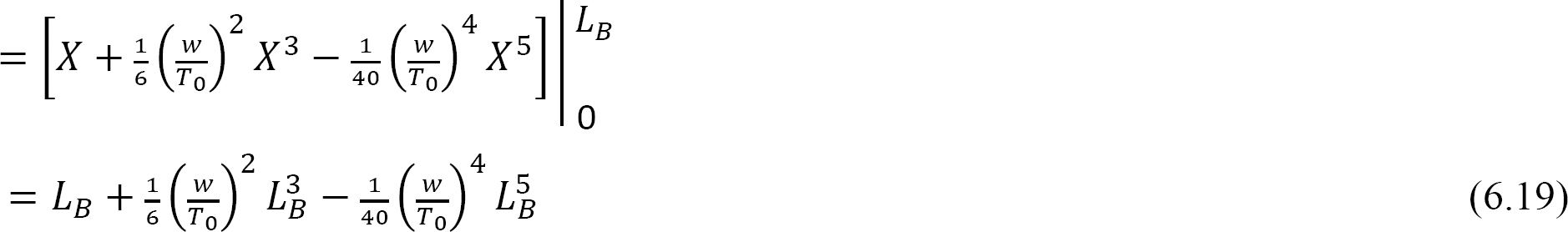
Putting 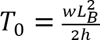 into equation 6.19 suggests:
Example 6.8
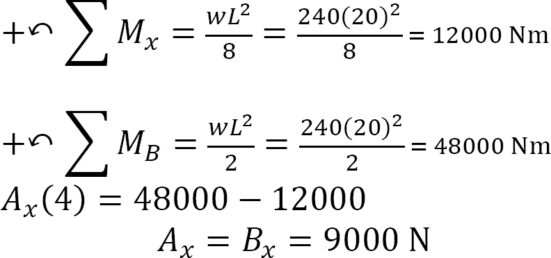
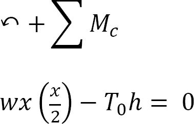
A cable subjected to a uniform load of 240 N/m is suspended between two supports at the same level 20 m apart, as shown in Figure 6.12. If the cable has a central sag of 4 m, determine the horizontal reactions at the supports, the minimum and maximum tension in the cable, and the total length of the cable.

Solution
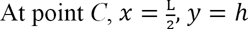
Horizontal reactions. Applying the general cable theorem at point C suggests the following:
when x =  ℎ = 4 m
Therefore, 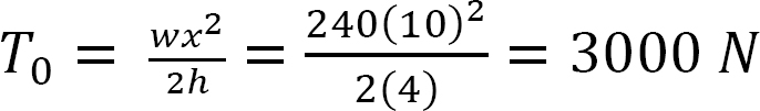
From equation 6.15, the maximum tension is found, as follows:

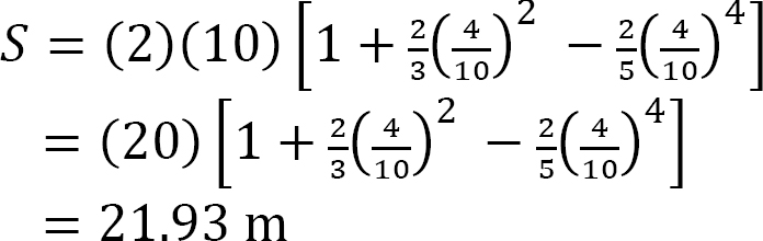
The total length of cable:
Chapter Summary
Internal forces in arches and cables: Arches are aesthetically pleasant structures consisting of curvilinear members. They are used for large-span structures. The presence of horizontal thrusts at the supports of arches results in the reduction of internal forces in it members. The lesser shear forces and bending moments at any section of the arches results in smaller member sizes and a more economical design compared with beam design.
Arches: Arches can be classified as two-pinned arches, three-pinned arches, or fixed arches based on their support and connection of members, as well as parabolic, segmental, or circular based on their shapes. Arches can also be classified as determinate or indeterminate. Three-pinned arches are determinate, while two-pinned arches and fixed arches, as shown in Figure 6.1, are indeterminate structures.
Cables: Cables are flexible structures in pure tension. They are used in different engineering applications, such as bridges and offshore platforms. They take different shapes, depending on the type of loading. Under concentrated loads, they take the form of segments between the loads, while under uniform loads, they take the shape of a curve, as shown below.
Some numerical examples have been solved in this chapter to demonstrate the procedures and theorem for the analysis of arches and cables.
Practice Problems
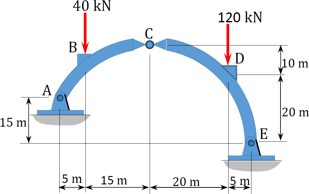
6.1 Determine the reactions at supports B and E of the three-hinged circular arch shown in Figure P6.1.
6.2 Determine the reactions at supports A and B of the parabolic arch shown in Figure P6.2. Also draw the bending moment diagram for the arch.

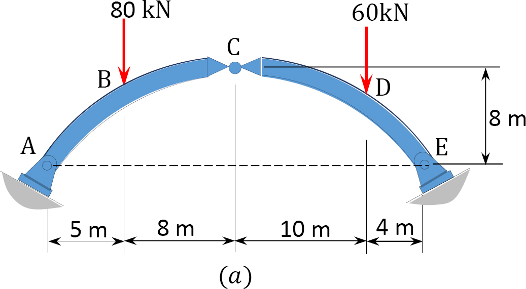
6.3 Determine the shear force, axial force, and bending moment at a point under the 80 kN load on the parabolic arch shown in Figure P6.3.
6.4 In Figure P6.4, a cable supports loads at point B and C. Determine the sag at point C and the maximum tension in the cable.
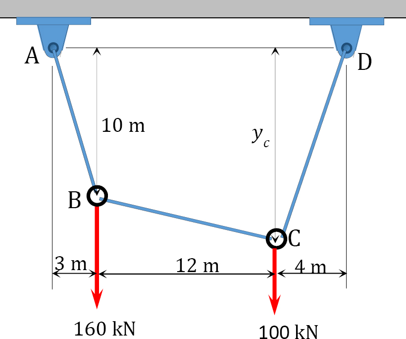
6.5 A cable supports three concentrated loads at points B, C, and D in Figure P6.5. Determine the total length of the cable and the length of each segment.

6.6 A cable is subjected to the loading shown in Figure P6.6. Determine the total length of the cable and the tension at each support.

6.7 A cable shown in Figure P6.7 supports a uniformly distributed load of 100 kN/m. Determine the tensions at supports A and C at the lowest point B.

6.8 A cable supports a uniformly distributed load in Figure P6.8. Find the horizontal reaction at the supports of the cable, the equation of the shape of the cable, the minimum and maximum tension in the cable, and the length of the cable.

6.9 A cable subjected to a uniform load of 300 N/m is suspended between two supports at the same level 20 m apart, as shown in Figure P6.9. If the cable has a central sag of 3 m, determine the horizontal reactions at the supports, the minimum and maximum tension in the cable, and the total length of the cable.
