12.3: ODEs in Two Dimensions

So far we’ve used ode45 to solve a system of first-order equations and a single second-order equation. Now we’ll take one more step, solving a system of second-order equations.

As an example, we’ll simulate the flight of a baseball. If there is no wind and no spin on the ball, the ball travels in a vertical plane, so we can think of the system as two-dimensional, with \(x\) representing the horizontal distance traveled from the starting place and \(y\) representing height or altitude.

Listing 12.1 shows a rate function we can use to simulate this system with ode45:

Listing 12.1: A rate function we can use to model the flight of a baseball

function res = rate_func(t, W)
    P = W(1:2);
    V = W(3:4);

    dPdt = V;
    dVdt = acceleration(t, P, V);

    res = [dPdt; dVdt];
end

function res = acceleration(t, P, V)
    g = 9.8;             % acceleration due to gravity in m/s^2
    a_gravity = [0; -g];
    res = a_gravity;
end

The second argument of rate_func is understood to be a vector, W, with four elements. The first two are assigned to P, which represents position; the last two are assigned to V, which represents velocity. Both P and V have two elements, representing the \(x\) and \(y\) components.

The goal of the rate function is to compute the derivative of W, so the output has to be a vector with four elements, where the first two represent the derivative of P and the last two represent the derivative of V. The derivative of P is velocity. We don’t have to compute it; we were given it as part of W. The derivative of V is acceleration. To compute it, we call acceleration, which takes as input variables time, position, and velocity. In this example, we don’t use any of the input variables, but we will soon.

For now we’ll ignore air resistance, so the only force on the baseball is gravity. We represent acceleration due to gravity with a vector that has magnitude g and direction along the negative y-axis.

Let’s assume that a ball is batted from an initial position 1 m above the home plate, with an initial velocity of 40 m/s in the horizontal and 30 m/s in the vertical direction.

Here’s how we can call ode45 with these initial conditions:

    P = [0; 1];       % initial position in m
    V = [40; 30];     % initial velocity in m/s
    W = [P; V];       % initial condition

    tspan = [0 8]
    [T, M] = ode45(@rate_func, tspan, W);

P and V are column vectors because we put semicolons between the elements. So W is a column vector with four elements. And tspan specifies that we want to run the simulation for 8 s.

The output variables from ode45 are a vector, T, that contains time values and a matrix, M, with four columns: the first two are position; the last two are velocity.

Here’s how we can plot position as a function of time:

    X = M(:, 1);
    Y = M(:, 2);

    plot(T, X)
    plot(T, Y)

X and Y get the first and second columns from M, which are the \(x\) and \(y\) position coordinates.

Figure 12.2 shows what these coordinates look like as a function of time. The x-coordinate increases linearly because the \(x\) velocity is constant. The y-coordinate goes up and down, as we expect.

Figure 12.2: Simulated flight of a baseball neglecting drag force

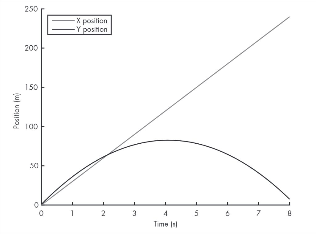
The simulation ends just before the ball lands, having traveled almost 250 m. That’s substantially farther than a real baseball would travel, because we have ignored air resistance, or “drag force.”