Engineering LibreTexts

12.4: Drag Force

  • Page ID
    84747
  • \( \newcommand{\vecs}[1]{\overset { \scriptstyle \rightharpoonup} {\mathbf{#1}} } \)

    \( \newcommand{\vecd}[1]{\overset{-\!-\!\rightharpoonup}{\vphantom{a}\smash {#1}}} \)

    \( \newcommand{\id}{\mathrm{id}}\) \( \newcommand{\Span}{\mathrm{span}}\)

    ( \newcommand{\kernel}{\mathrm{null}\,}\) \( \newcommand{\range}{\mathrm{range}\,}\)

    \( \newcommand{\RealPart}{\mathrm{Re}}\) \( \newcommand{\ImaginaryPart}{\mathrm{Im}}\)

    \( \newcommand{\Argument}{\mathrm{Arg}}\) \( \newcommand{\norm}[1]{\| #1 \|}\)

    \( \newcommand{\inner}[2]{\langle #1, #2 \rangle}\)

    \( \newcommand{\Span}{\mathrm{span}}\)

    \( \newcommand{\id}{\mathrm{id}}\)

    \( \newcommand{\Span}{\mathrm{span}}\)

    \( \newcommand{\kernel}{\mathrm{null}\,}\)

    \( \newcommand{\range}{\mathrm{range}\,}\)

    \( \newcommand{\RealPart}{\mathrm{Re}}\)

    \( \newcommand{\ImaginaryPart}{\mathrm{Im}}\)

    \( \newcommand{\Argument}{\mathrm{Arg}}\)

    \( \newcommand{\norm}[1]{\| #1 \|}\)

    \( \newcommand{\inner}[2]{\langle #1, #2 \rangle}\)

    \( \newcommand{\Span}{\mathrm{span}}\) \( \newcommand{\AA}{\unicode[.8,0]{x212B}}\)

    \( \newcommand{\vectorA}[1]{\vec{#1}}      % arrow\)

    \( \newcommand{\vectorAt}[1]{\vec{\text{#1}}}      % arrow\)

    \( \newcommand{\vectorB}[1]{\overset { \scriptstyle \rightharpoonup} {\mathbf{#1}} } \)

    \( \newcommand{\vectorC}[1]{\textbf{#1}} \)

    \( \newcommand{\vectorD}[1]{\overrightarrow{#1}} \)

    \( \newcommand{\vectorDt}[1]{\overrightarrow{\text{#1}}} \)

    \( \newcommand{\vectE}[1]{\overset{-\!-\!\rightharpoonup}{\vphantom{a}\smash{\mathbf {#1}}}} \)

    \( \newcommand{\vecs}[1]{\overset { \scriptstyle \rightharpoonup} {\mathbf{#1}} } \)

    \( \newcommand{\vecd}[1]{\overset{-\!-\!\rightharpoonup}{\vphantom{a}\smash {#1}}} \)

    \(\newcommand{\avec}{\mathbf a}\) \(\newcommand{\bvec}{\mathbf b}\) \(\newcommand{\cvec}{\mathbf c}\) \(\newcommand{\dvec}{\mathbf d}\) \(\newcommand{\dtil}{\widetilde{\mathbf d}}\) \(\newcommand{\evec}{\mathbf e}\) \(\newcommand{\fvec}{\mathbf f}\) \(\newcommand{\nvec}{\mathbf n}\) \(\newcommand{\pvec}{\mathbf p}\) \(\newcommand{\qvec}{\mathbf q}\) \(\newcommand{\svec}{\mathbf s}\) \(\newcommand{\tvec}{\mathbf t}\) \(\newcommand{\uvec}{\mathbf u}\) \(\newcommand{\vvec}{\mathbf v}\) \(\newcommand{\wvec}{\mathbf w}\) \(\newcommand{\xvec}{\mathbf x}\) \(\newcommand{\yvec}{\mathbf y}\) \(\newcommand{\zvec}{\mathbf z}\) \(\newcommand{\rvec}{\mathbf r}\) \(\newcommand{\mvec}{\mathbf m}\) \(\newcommand{\zerovec}{\mathbf 0}\) \(\newcommand{\onevec}{\mathbf 1}\) \(\newcommand{\real}{\mathbb R}\) \(\newcommand{\twovec}[2]{\left[\begin{array}{r}#1 \\ #2 \end{array}\right]}\) \(\newcommand{\ctwovec}[2]{\left[\begin{array}{c}#1 \\ #2 \end{array}\right]}\) \(\newcommand{\threevec}[3]{\left[\begin{array}{r}#1 \\ #2 \\ #3 \end{array}\right]}\) \(\newcommand{\cthreevec}[3]{\left[\begin{array}{c}#1 \\ #2 \\ #3 \end{array}\right]}\) \(\newcommand{\fourvec}[4]{\left[\begin{array}{r}#1 \\ #2 \\ #3 \\ #4 \end{array}\right]}\) \(\newcommand{\cfourvec}[4]{\left[\begin{array}{c}#1 \\ #2 \\ #3 \\ #4 \end{array}\right]}\) \(\newcommand{\fivevec}[5]{\left[\begin{array}{r}#1 \\ #2 \\ #3 \\ #4 \\ #5 \\ \end{array}\right]}\) \(\newcommand{\cfivevec}[5]{\left[\begin{array}{c}#1 \\ #2 \\ #3 \\ #4 \\ #5 \\ \end{array}\right]}\) \(\newcommand{\mattwo}[4]{\left[\begin{array}{rr}#1 \amp #2 \\ #3 \amp #4 \\ \end{array}\right]}\) \(\newcommand{\laspan}[1]{\text{Span}\{#1\}}\) \(\newcommand{\bcal}{\cal B}\) \(\newcommand{\ccal}{\cal C}\) \(\newcommand{\scal}{\cal S}\) \(\newcommand{\wcal}{\cal W}\) \(\newcommand{\ecal}{\cal E}\) \(\newcommand{\coords}[2]{\left\{#1\right\}_{#2}}\) \(\newcommand{\gray}[1]{\color{gray}{#1}}\) \(\newcommand{\lgray}[1]{\color{lightgray}{#1}}\) \(\newcommand{\rank}{\operatorname{rank}}\) \(\newcommand{\row}{\text{Row}}\) \(\newcommand{\col}{\text{Col}}\) \(\renewcommand{\row}{\text{Row}}\) \(\newcommand{\nul}{\text{Nul}}\) \(\newcommand{\var}{\text{Var}}\) \(\newcommand{\corr}{\text{corr}}\) \(\newcommand{\len}[1]{\left|#1\right|}\) \(\newcommand{\bbar}{\overline{\bvec}}\) \(\newcommand{\bhat}{\widehat{\bvec}}\) \(\newcommand{\bperp}{\bvec^\perp}\) \(\newcommand{\xhat}{\widehat{\xvec}}\) \(\newcommand{\vhat}{\widehat{\vvec}}\) \(\newcommand{\uhat}{\widehat{\uvec}}\) \(\newcommand{\what}{\widehat{\wvec}}\) \(\newcommand{\Sighat}{\widehat{\Sigma}}\) \(\newcommand{\lt}{<}\) \(\newcommand{\gt}{>}\) \(\newcommand{\amp}{&}\) \(\definecolor{fillinmathshade}{gray}{0.9}\)

    A simple model for the drag force on a baseball is

    \[\textbf{F}_\mathrm{d} = - \frac{1}{2} \, \rho v C_\mathrm{d} A \hat{\textbf{V}}\notag \]

    where \(\textbf{F}_\mathrm{d}\) is a vector that represents the force on the baseball due to drag, \(\rho\) is the density of air, \(C_\mathrm{d}\) is the drag coefficient, and \(A\) is the cross-sectional area.

    \(\textbf{V}\) is the baseball’s velocity vector, \(v\) is the magnitude of \(\textbf{V}\), and \(\hat{\textbf{V}}\) is a unit vector in the same direction as \(\textbf{V}\). The minus sign at the beginning means that the result is in the opposite direction to \(\textbf{V}\).

    The function in Listing 12.2 computes the drag force on a baseball:

    Listing 12.2: A function that calculates the drag force on a baseball

     function res = drag_force(V)
        C_d = 0.3;      % dimensionless
        rho = 1.3;      % kg / m^3
        A = 0.0042;     % m^2
        v = norm(V);    % m/s
    
        res = -1/2 * C_d * rho * A * v * V;
    end

    The drag coefficient for a baseball is about 0.3. The density of air at sea level is about 1.3 kg/m3. The cross-sectional area of a baseball is 0.0042 m2.

    Now we have to update acceleration to take drag into account:

    function res = acceleration(t, P, V)
        g = 9.8;                       % acceleration due to gravity in m/s^2
        a_gravity = [0; -g];
    
        m = 0.145;                     % mass in kilograms
        a_drag = drag_force(V) / m;
        res = a_gravity + a_drag;
    end

    As in Listing 12.1, acceleration represents acceleration due to gravity with a vector that has magnitude g and direction along the negative y-axis. But now it also computes drag force and divides by the mass of the baseball to get acceleration due to drag. Finally, it adds a_gravity and a_drag to get the total acceleration of the baseball.

    Figure 12.3 shows the following quantities graphically: (1) acceleration due to drag, \(\textbf{D}\), which is in the opposite direction to (2) velocity, \(\textbf{V}\); (3) acceleration due to gravity, \(\textbf{G}\), which is straight down; and (4) total acceleration, \(\textbf{A}\), which is the sum of \(\textbf{D}\) and \(\textbf{G}\).

    12.3.jpg
    Figure 12.3: Diagram of velocity, \(\textbf{V}\); acceleration due to drag force, \(\textbf{D}\); acceleration due to gravity, \(\textbf{G}\); and total acceleration, \(\textbf{A}\)

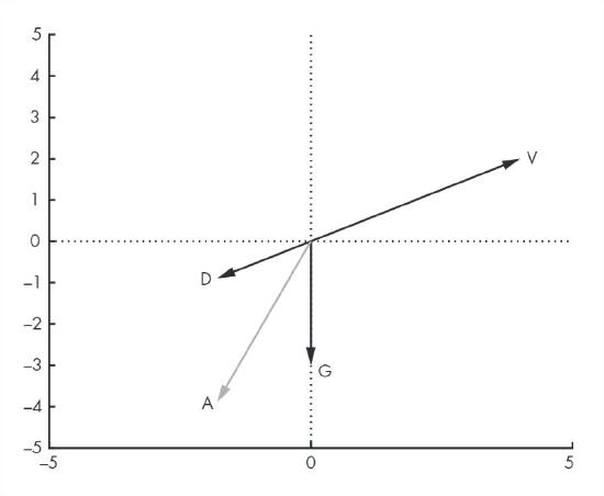
    Figure 12.4 shows the results from ode45. The ball lands after about 5 s, having traveled less than 150 m, substantially less than what we got without air resistance, about 250 m.

    12.4.jpg
    Figure 12.4: Simulated flight of a baseball including drag force

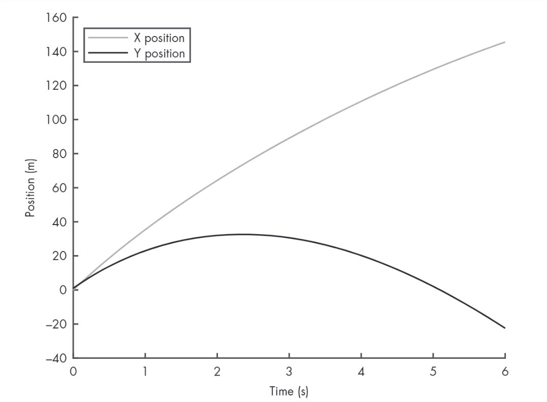
    This result suggests that ignoring air resistance is not a good choice for modeling a baseball.


    This page titled 12.4: Drag Force is shared under a CC BY-NC 4.0 license and was authored, remixed, and/or curated by Allen B. Downey (Green Tea Press) via source content that was edited to the style and standards of the LibreTexts platform.