9.29: The Mathematics of the Sine Function
- Page ID
- 14649
\( \newcommand{\vecs}[1]{\overset { \scriptstyle \rightharpoonup} {\mathbf{#1}} } \)
\( \newcommand{\vecd}[1]{\overset{-\!-\!\rightharpoonup}{\vphantom{a}\smash {#1}}} \)
\( \newcommand{\id}{\mathrm{id}}\) \( \newcommand{\Span}{\mathrm{span}}\)
( \newcommand{\kernel}{\mathrm{null}\,}\) \( \newcommand{\range}{\mathrm{range}\,}\)
\( \newcommand{\RealPart}{\mathrm{Re}}\) \( \newcommand{\ImaginaryPart}{\mathrm{Im}}\)
\( \newcommand{\Argument}{\mathrm{Arg}}\) \( \newcommand{\norm}[1]{\| #1 \|}\)
\( \newcommand{\inner}[2]{\langle #1, #2 \rangle}\)
\( \newcommand{\Span}{\mathrm{span}}\)
\( \newcommand{\id}{\mathrm{id}}\)
\( \newcommand{\Span}{\mathrm{span}}\)
\( \newcommand{\kernel}{\mathrm{null}\,}\)
\( \newcommand{\range}{\mathrm{range}\,}\)
\( \newcommand{\RealPart}{\mathrm{Re}}\)
\( \newcommand{\ImaginaryPart}{\mathrm{Im}}\)
\( \newcommand{\Argument}{\mathrm{Arg}}\)
\( \newcommand{\norm}[1]{\| #1 \|}\)
\( \newcommand{\inner}[2]{\langle #1, #2 \rangle}\)
\( \newcommand{\Span}{\mathrm{span}}\) \( \newcommand{\AA}{\unicode[.8,0]{x212B}}\)
\( \newcommand{\vectorA}[1]{\vec{#1}} % arrow\)
\( \newcommand{\vectorAt}[1]{\vec{\text{#1}}} % arrow\)
\( \newcommand{\vectorB}[1]{\overset { \scriptstyle \rightharpoonup} {\mathbf{#1}} } \)
\( \newcommand{\vectorC}[1]{\textbf{#1}} \)
\( \newcommand{\vectorD}[1]{\overrightarrow{#1}} \)
\( \newcommand{\vectorDt}[1]{\overrightarrow{\text{#1}}} \)
\( \newcommand{\vectE}[1]{\overset{-\!-\!\rightharpoonup}{\vphantom{a}\smash{\mathbf {#1}}}} \)
\( \newcommand{\vecs}[1]{\overset { \scriptstyle \rightharpoonup} {\mathbf{#1}} } \)
\( \newcommand{\vecd}[1]{\overset{-\!-\!\rightharpoonup}{\vphantom{a}\smash {#1}}} \)
\(\newcommand{\avec}{\mathbf a}\) \(\newcommand{\bvec}{\mathbf b}\) \(\newcommand{\cvec}{\mathbf c}\) \(\newcommand{\dvec}{\mathbf d}\) \(\newcommand{\dtil}{\widetilde{\mathbf d}}\) \(\newcommand{\evec}{\mathbf e}\) \(\newcommand{\fvec}{\mathbf f}\) \(\newcommand{\nvec}{\mathbf n}\) \(\newcommand{\pvec}{\mathbf p}\) \(\newcommand{\qvec}{\mathbf q}\) \(\newcommand{\svec}{\mathbf s}\) \(\newcommand{\tvec}{\mathbf t}\) \(\newcommand{\uvec}{\mathbf u}\) \(\newcommand{\vvec}{\mathbf v}\) \(\newcommand{\wvec}{\mathbf w}\) \(\newcommand{\xvec}{\mathbf x}\) \(\newcommand{\yvec}{\mathbf y}\) \(\newcommand{\zvec}{\mathbf z}\) \(\newcommand{\rvec}{\mathbf r}\) \(\newcommand{\mvec}{\mathbf m}\) \(\newcommand{\zerovec}{\mathbf 0}\) \(\newcommand{\onevec}{\mathbf 1}\) \(\newcommand{\real}{\mathbb R}\) \(\newcommand{\twovec}[2]{\left[\begin{array}{r}#1 \\ #2 \end{array}\right]}\) \(\newcommand{\ctwovec}[2]{\left[\begin{array}{c}#1 \\ #2 \end{array}\right]}\) \(\newcommand{\threevec}[3]{\left[\begin{array}{r}#1 \\ #2 \\ #3 \end{array}\right]}\) \(\newcommand{\cthreevec}[3]{\left[\begin{array}{c}#1 \\ #2 \\ #3 \end{array}\right]}\) \(\newcommand{\fourvec}[4]{\left[\begin{array}{r}#1 \\ #2 \\ #3 \\ #4 \end{array}\right]}\) \(\newcommand{\cfourvec}[4]{\left[\begin{array}{c}#1 \\ #2 \\ #3 \\ #4 \end{array}\right]}\) \(\newcommand{\fivevec}[5]{\left[\begin{array}{r}#1 \\ #2 \\ #3 \\ #4 \\ #5 \\ \end{array}\right]}\) \(\newcommand{\cfivevec}[5]{\left[\begin{array}{c}#1 \\ #2 \\ #3 \\ #4 \\ #5 \\ \end{array}\right]}\) \(\newcommand{\mattwo}[4]{\left[\begin{array}{rr}#1 \amp #2 \\ #3 \amp #4 \\ \end{array}\right]}\) \(\newcommand{\laspan}[1]{\text{Span}\{#1\}}\) \(\newcommand{\bcal}{\cal B}\) \(\newcommand{\ccal}{\cal C}\) \(\newcommand{\scal}{\cal S}\) \(\newcommand{\wcal}{\cal W}\) \(\newcommand{\ecal}{\cal E}\) \(\newcommand{\coords}[2]{\left\{#1\right\}_{#2}}\) \(\newcommand{\gray}[1]{\color{gray}{#1}}\) \(\newcommand{\lgray}[1]{\color{lightgray}{#1}}\) \(\newcommand{\rank}{\operatorname{rank}}\) \(\newcommand{\row}{\text{Row}}\) \(\newcommand{\col}{\text{Col}}\) \(\renewcommand{\row}{\text{Row}}\) \(\newcommand{\nul}{\text{Nul}}\) \(\newcommand{\var}{\text{Var}}\) \(\newcommand{\corr}{\text{corr}}\) \(\newcommand{\len}[1]{\left|#1\right|}\) \(\newcommand{\bbar}{\overline{\bvec}}\) \(\newcommand{\bhat}{\widehat{\bvec}}\) \(\newcommand{\bperp}{\bvec^\perp}\) \(\newcommand{\xhat}{\widehat{\xvec}}\) \(\newcommand{\vhat}{\widehat{\vvec}}\) \(\newcommand{\uhat}{\widehat{\uvec}}\) \(\newcommand{\what}{\widehat{\wvec}}\) \(\newcommand{\Sighat}{\widehat{\Sigma}}\) \(\newcommand{\lt}{<}\) \(\newcommand{\gt}{>}\) \(\newcommand{\amp}{&}\) \(\definecolor{fillinmathshade}{gray}{0.9}\)def getBounceAmount(currentBounce, bounceRate, bounceHeight): # Returns the number of pixels to offset based on the bounce. # Larger bounceRate means a slower bounce. # Larger bounceHeight means a higher bounce. # currentBounce will always be less than bounceRate return int(math.sin( (math.pi / float(bounceRate)) * currentBounce ) * bounceHeight)
There is a mathematical function (which is similar to functions in programming in that they both "return" or "evaluate" to a number based on their parameters) called sine (pronounced like "sign" and often abbreviated as "sin"). You may have learned about it in math class, but if you haven’t it will be explained here. Python has this mathematic function as a Python function in the math
module. You can pass an int or float value to math.sin()
, and it will return a float value that is called the "sine value"
In the interactive shell, let’s see what math.sin()
returns for some values:
>>> import math >>> math.sin(1) 0.8414709848078965 >>> math.sin(2) 0.90929742682568171 >>> math.sin(3) 0.14112000805986721 >>> math.sin(4) -0.7568024953079282 >>> math.sin(5) -0.95892427466313845
It seems really hard to predict what value math.sin()
is going to return based on what value we pass it (which might make you wonder what math.sin()
is useful for). But if we graph the sine values of the integers 1
through 10
on a graph, we would get this:
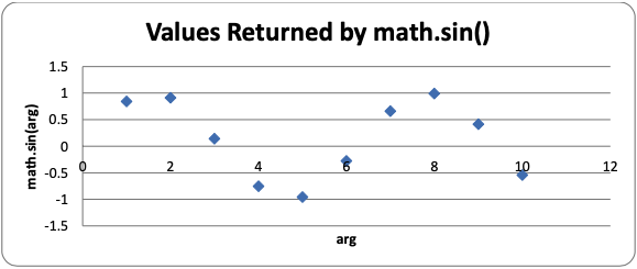
You can kind of see a wavy pattern in the values returned by math.sin()
. If you figure out the sine values for more numbers besides integers (for example, 1.5
and 2.5
and so on) and then connect the dots with lines, you can see this wavy pattern more easily:
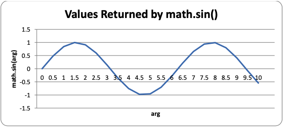
In fact, if you kept adding more and more data points to this graph, you would see that the sine wave looks like this:
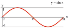
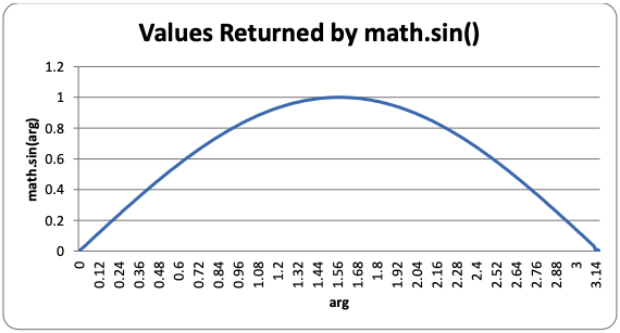
Notice that math.sin(0)
returns 0
, then gradually increases until math.sin(3.14 / 2)
returns 1
, then it begins to decrease until math.sin(3.14)
returns 0
. The number 3.14
is a special number in mathematics called pi (pronounced the same as delicious "pie"). This value is also stored in the constant variable pi
in the math
module (which is why line 6 [333] uses the variable, math.pi
), which is technically the float value 3.1415926535897931
. Since we want a wavy-looking bounce for our squirrel, we’ll only pay attention to the return values of math.sin()
for the arguments 0
to 3.14
:
Let’s take a look at the return value of getBounceAmount()
and figure out what it does exactly.
Remember that on line 21 we set the BOUNCERATE
constant to 6
. This means that our code will only increment playerObj['bounce']
from 0
to 6
and that we want to split up the range of floating-point values from 0
to 3.14
into 6 parts, which we can do with simple division: 3.14 / 6 = 0.5235
. Each of the 6 equal parts of the 3.14
length on the graph for the "sine wave bounce" is 0.5235
.
You can see that when playerObj['bounce']
is at 3
(halfway between 0
and 6
), the value passed to the math.sin()
call is math.pi / 6 * 3
, which is 1.5707
(halfway between 0
and 3.1415
). Then math.sin(1.5707)
will return 1.0
, which is the highest part of the sine wave (and the highest part of the sine wave happens half way through the wave).
As playerObj['bounce']
gets its value incremented, the getBounceAmount()
function will return values that have the same bounce shape that the sine wave has from 0
to 3.14
. If you want to make the bounce higher, than increase the BOUNCEHEIGHT
constant. If you want to make the bounce slower, than increase the BOUNCERATE
constant.
The sine function is a concept from trigonometry mathematics. If you’d like to learn more about the sine wave, the Wikipedia page has detailed information: http://en.Wikipedia.org/wiki/Sine.