1.1: Activity 1 - Overview of Algorithm Design and Analysis

Introduction

There are compelling reasons to study algorithms. To put it simply, computer programs would not exist without algorithms. And with computer applications becoming indispensable in almost all aspects of our professional and personal lives, studying algorithms becomes a necessity for more and more people.

Another reason for studying algorithms is their usefulness in developing analytical skills. After all, algorithms can be seen as special kinds of solutions to problems, not answers but precisely defined procedures for getting answers. Consequently, specific algorithm design techniques can be interpreted as problem solving strategies that can be useful regardless of whether a computer is involved.

Activity Details

The term algorithm can be defined using any of the following statements:

• An algorithm is a set of rules for carrying out calculation either by hand or on a machine.

• An algorithm is a finite step-by-step procedure to achieve a required result.

• An algorithm is a sequence of computational steps that transform the input into the output.

• An algorithm is a sequence of operations performed on data that have to be organized in data structures.

• An algorithm is an abstraction of a program to be executed on a physical machine (model of Computation).

The most famous algorithm in history dates well before the time of the ancient Greeks: this is the Euclid’s algorithm for calculating the greatest common divisor of two integers.

The Classic Multiplication Algorithm

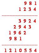
Multiplication, the American way:

Multiply the multiplicand one after another by each digit of the multiplier taken from right to left.

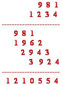
Multiplication, the English way:

Multiply the multiplicand one after another by each digit of the multiplier taken from left to right.

Algorithmics is a branch of computer science that consists of designing and analyzing computer algorithms.

The “design” concern to:

• The description of algorithm at an abstract level by means of a pseudo language, and

• Proof of correctness that is, the algorithm solves the given problem in all cases.

The “analysis” deals with performance evaluation (complexity analysis).

We start with defining the model of computation, which is usually the Random Access Machine (RAM) model, but other models of computations can be use such as PRAM. Once the model of computation has been defined, an algorithm can be describe using a simple language (or pseudo language) whose syntax is close to programming language such as C or java.

Algorithm’s Performance

Two important ways to characterize the effectiveness of an algorithm are its space complexity and time complexity. Time complexity of an algorithm concerns with determining an expression of the number of steps needed as a function of the problem size. Since the step count measure is somewhat rough, one does not aim at obtaining an exact step count. Instead, one attempts only to get asymptotic bounds on the step count.

Asymptotic analysis makes use of the O (Big Oh) notation. Two other notational constructs used by computer scientists in the analysis of algorithms are Θ (Big Theta) notation and Ω (Big Omega) notation. The performance evaluation of an algorithm is obtained by tallying the number of occurrences of each operation when running the algorithm. The performance of an algorithm is evaluated as a function of the input size n and is to be considered modulo a multiplicative constant.

The following notations are commonly use notations in performance analysis and used to characterize the complexity of an algorithm.

Θ-Notation (Same order)

This notation bounds a function to within constant factors. We say f(n) = Θ(g(n)) if there exist positive constants n0, c1 and c2 such that to the right of n0 the value of f(n) always lies between c1 g(n) and c2 g(n) inclusive.

In the set notation, we write as follows:

Θ(g(n)) = {f(n) : there exist positive constants c1, c2, and n0 such that 0 ≤ c1 g(n) ≤ f(n) ≤ c2 g(n) for all n ≥ n0}

We say that g(n) is an asymptotically tight bound for f(n)

Figure 1.1.1 : Graphs to demonstrate Θ(g(n))

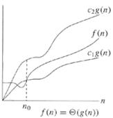
As shown in Figure 1.1.1 , graphically, for all values of n to the right of n0, the value of f(n) lies at or above c1 g(n) and at or below c2 g(n). In other words, for all n ≥ n0, the function f(n) is equal to g(n) to within a constant factor. We say that g(n) is an asymptotically tight bound for f(n).

In the set terminology, f(n) is said to be a member of the set Θ(g(n)) of functions. In other words, because O(g(n)) is a set, we could write

f(n) ∈ Θ(g(n))

to indicate that f(n) is a member of Θ(g(n)). Instead, we write

f(n) = Θ(g(n))

to express the same notation.

Historically, this notation is “f(n) = Θ(g(n))” although the idea that f(n) is equal to something called Θ(g(n)) is misleading.

Example: n2/2 − 2n = Θ(n2), with c1 = 1/4, c2 = 1/2, and n0 = 8.

Ο-Notation (Upper Bound)

This notation gives an upper bound for a function to within a constant factor. We write f(n) = O(g(n)) if there are positive constants n0 and c such that to the right of n0, the value of f(n) always lies on or below c g(n).

In the set notation, we write as follows: For a given function g(n), the set of functions

Ο(g(n)) = {f(n): there exist positive constants c and n0 such that 0 ≤ f(n) ≤ c g(n) for all n ≥ n0}

We say that the function g(n) is an asymptotic upper bound for the function f(n). We use Ο-notation to give an upper bound on a function, to within a constant factor.

Figure 1.1.2 : Graphs to demonstrate O(g(n))

As shown in Figure 1.1.2 , graphically, for all values of n to the right of n0, the value of the function f(n) is on or below g(n). We write f(n) = O(g(n)) to indicate that a function f(n) is a member of the set Ο(g(n)) i.e.

f(n) ∈ Ο(g(n))

Note that f(n) = Θ(g(n)) implies f(n) = Ο(g(n)), since Θ-notation is a stronger notation than Ο-notation.

Example: 2n2 = Ο(n3), with c = 1 and n0 = 2.

Equivalently, we may also define f is of order g as follows:

If f(n) and g(n) are functions defined on the positive integers, then f(n) is Ο(g(n)) if and only if there is a c > 0 and an n0 > 0 such that

| f(n) | ≤ | g(n) | for all n ≥ n0

Ω-Notation (Lower Bound)

This notation gives a lower bound for a function to within a constant factor. We write f(n) = Ω(g(n)) if there are positive constants n0 and c such that to the right of n0, the value of f(n) always lies on or above c g(n).

In the set notation, we write as follows: For a given function g(n), the set of functions

Ω(g(n)) = {f(n) : there exist positive constants c and n0 such that 0 ≤ c g(n) ≤ f(n) for all n ≥ n0}

We say that the function g(n) is an asymptotic lower bound for the function f(n).

Figure 1.1.3 : Graphs to demonstrate Ω(g(n))

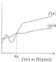
Figure 1.1.3 provides an insight behind Ω-notation. For example, √n = (lg n), with c = 1 and n0 = 16.

Algorithm’s Analysis

The complexity of an algorithm is a function g(n) that gives the upper bound of the number of operation (or running time) performed by an algorithm when the input size is n.

There are two interpretations of upper bound.

• Worst-case Complexity: the running time for any given size input will be lower than the upper bound except possibly for some values of the input where the maximum is reached.
• Average-case Complexity: the running time for any given size input will be the average number of operations over all problem instances for a given size.

Because it is quite difficult to estimate the statistical behaviour of the input, most of the time we content ourselves to a worst case behaviour. Most of the time, the complexity of g(n) is approximated by its family O(f(n)) where f(n) is one of the following functions: n (linear complexity), log n (logarithmic complexity), na where a ≥ 2 (polynomial complexity), an (exponential complexity).

Optimality

Once the complexity of an algorithm has been estimated, the question arises whether this algorithm is optimal. An algorithm for a given problem is optimal if its complexity reaches the lower bound over all the algorithms solving this problem. For example, any algorithm solving “the intersection of n segments” problem will execute at least n2 operations in the worst case even if it does nothing but print the output. This is abbreviated by saying that the problem has Ω(n2) complexity. If one finds an O(n2) algorithm that solves this problem, it will be optimal and of complexity Θ(n2).

Reduction

Another technique for estimating the complexity of a problem is the transformation of problems, also called problem reduction. As an example, suppose we know a lower bound for a problem A, and that we would like to estimate a lower bound for a problem B. If we can transform A into B by a transformation step whose cost is less than that for solving A, then B has the same bound as A.

The Convex hull problem nicely illustrates “reduction” technique. A lower bound of Convex-hull problem is established by reducing the sorting problem (complexity: Θ(n log n)) to the Convex hull problem.

Conclusion

This activity introduced the basic concepts of algorithm design and analysis. The need for analysing the time and space complexity of algorithms was articulated and the notations for describing algorithm complexity were presented.

Assessment

1. Distinguish between space and time complexity.

2. Briefly explain the commonly used notations in performance analysis.