1.2: Activity 2 - Recursion and Recursive Backtracking

Introduction

Recursion and backtracking are important problem solving approaches, which are alternative to iteration. An iterative solution involves loops. Not all recursive solutions are better than iterative solutions, though. Some recursive solutions may be impractical because they are so inefficient. Nevertheless, recursion can provide elegantly simple solutions to problems of great complexity.

Activity Details

When we encounter a problem that requires repetition, we often use iteration, that is, some form of loop structures. Iterative problems include the problem of printing a series of integers from n1 to n2, where n1 <= n2, whose iterative solution is presented below:

void printSeries(int n1, int n2) {
for (int i = n1; i < n2; i++) {
    print(i + “, “);}
println(n2);

An alternative approach to problems that require repetition is to solve them using recursion. A recursive method is a method that calls itself. Applying this approach to the print-series problem gives the following algorithm:

void printSeries(int n1, int n2) {
if (n1 == n2) {
println(n2);}
else {
    print(n1 + “, “);
    printSeries(n1 + 1, n2);}

Considering the recursive approach above the following is the trace for the method call

printSeries(5, 7):
printSeries(5, 7):
print(5 + “, “);
printSeries(6, 7):
print(6 + “, “);
printSeries(7, 7):
print(7);
return
return
return

When we use recursion, we solve a problem by reducing it to a simpler problem of the same kind. We keep doing this until we reach a problem that is simple enough to be solved directly. This simplest problem is known as the base case. The base case stops the recursion, because it doesn’t make another call to the method. In the printSeries function, the base case is when n1 and n2 are equal and the if block executes.

If the base case hasn’t been reached, the recursive case is executed. In the printSeries function, the recursive case is when n1 and n2 are not equal and the else block executes. The recursive case reduces the overall problem to one or more simpler problems of the same kind and makes recursive calls to solve the simpler problems. The general Structure of a Recursive Method is presented below:

recursiveMethod(parameters) {
    if (stopping condition) {
// handle the base case
    } else {
// recursive case:
// possibly do something here
    recursiveMethod(modified parameters);
// possibly do something here}

Note that there may be multiple base cases and recursive cases. When we make the recursive call, we typically use parameters that bring us closer to a base case.

Consider the problem of Printing a File in Reverse Order. How can we print the lines of a file in reverse order? It’s not easy to do this using iteration. Why not? It’s easy to do it using recursion! A recursive function for printing lines of a file in reverse order is presented below:

void printRecursive(Scanner input) {
    if (!input.hasNextLine()) { // base case
    return;}
    String line = input.nextLine();
    println(line);
    printRecursive(input); // print the rest}

When using recursion care must be taken to avoid infinite recursion!! We have to ensure that a recursive method will eventually reach a base case, regardless of the initial input, otherwise, we can get infinite recursion which produces stack overflow, that is, there’s no room for more frames on the stack! Below is an example of our sum() method that its test for the base case can potentially cause infinite recursion. What values of n would cause infinite recursion?

int sum(int n) {
    if (n == 0) {
    return 0;}
    int total = n + sum(n – 1);
    return total;}

The philosophy for defining a recursive solution requires thinking recursively. That is when solving a problem using recursion, ask yourself these questions:

1. How can I break this problem down into one or more smaller subproblems and make recursive method calls to solve the subproblems?

2. What are the base cases? i.e., which subproblems are small enough to solve directly?

3. Do I need to combine the solutions to the subproblems? If so, how should I do so?

Recursive Backtracking

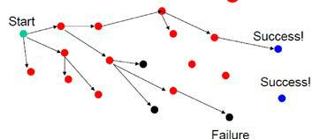
Recursive backtracking perceives that a problem solution space consists of states (nodes) and actions (paths that lead to new states). When in a node, can only see paths to connected nodes, thus if a node only leads to failure go back to its “parent” node and try other alternatives. If these all lead to failure then more backtracking may be necessary. Figure 1.2.1 presents such a tree modeled solution space.

Figure 1.2.1 : Different problem solution paths

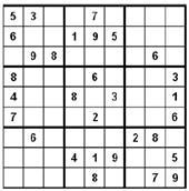
For example consider a Sudoku game of 9 by 9 matrixes with some numbers filled in, where all numbers must be between 1 and 9. The goal is that for each row, each column, and each mini matrix must contain the numbers between 1 and 9 once. That is no duplicates in rows, columns, or mini matrices are allowed. Figure 1.2.2 presents the initial game board.

Figure 1.2.2 : Initial Sudoku game board

Solving Sudoku by Brute Force - A brute force algorithm is a simple but general approach, and mainly performs the following two steps.

1. Try all combinations until you find one that works.

2. Then try and improve on the brute force results.

This approach isn’t clever, but computers are fast. The Sudoku Brute force Sudoku Solution can proceed by following steps.

1. If not open cells, solved

2. scan cells from left to right, top to bottom for first open cell

3. When an open cell is found start cycling through digits 1 to 9.

4. When a digit is placed check that the set up is legal

5. Now solve the board

Now, after placing a number in a cell is the remaining problem very similar to the original problem? Yes/No? Figure 1.2.3 shows a few such moves

Figure 1.2.3 : Making Brute-force moves

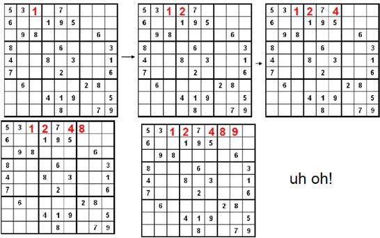
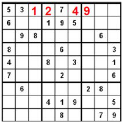
Unfortunately, the performed move reaches a dead end in our search. Note that with the current set up none of the nine digits work in the top right corner. When the search reaches a dead end, we would to back-up to the previous cell the algorithm was trying to fill and go onto to the next digit. In this case, the algorithm back up to the cell with 9 and that turns out to be a dead end as well, so should back up again (therefore, the algorithm needs to remember what digit to try next). Now in the cell with 8, we try 9 and move forward again as shown in Figure 1.2.4 .

Figure 1.2.4 : A back-up Replaces 8 with 9

The basic characteristics of Brute Force and Backtracking are:

• Brute force algorithms are slow

• They don’t employ a lot of logic - For example we know a 6 can’t go in the last 3 columns of the first row, but the brute force algorithm will plow ahead any way!

• But, brute force algorithms are fairly easy to implement as a first pass solution - many backtracking algorithms are brute force algorithms.

The following are the key insights when making use of the Brute Force and Backtracking:

• After trying placing a digit in a cell we want to solve the new sudoku board. Isn’t that a smaller (or simpler version) of the same problem we started with?

• After placing a number in a cell the we need to remember the next number to try in case things don’t work out.

• We need to know if things worked out (found a solution) or they didn’t, and if they didn’t try the next number

• If we try all numbers and none of them work in our cell we need to report back that things didn’t work

Problems such as Suduko can be solved using recursive backtracking. Recursive because later versions of the problem are just slightly simpler versions of the original. Backtracking because we may have to try different alternatives!

Pseudo code for recursive backtracking algorithms

1. If at a solution, report success

2. For every possible choice from current state / node

1. Make that choice and take one step along path

2. Use recursion to solve the problem for the new node / state

3. If the recursive call succeeds, report the success to the next lower level, otherwise, Back out of the current choice to restore the state at the beginning of the loop. Report failure

The following are possible goals of backtracking.

• Find a path to success

• Find all paths to success

• Find the best path to success

Figure 1.2.5 show a possible goal search space. Not all problems are exactly alike, and finding one success node may not be the end of the search.

Figure 1.2.5 : Possible goal solution space

The n-Queens Problem

Consider the n-Queens Problem whose goal is to find all possible ways of placing n queens on an n x n chessboard so that no two queens occupy the same row, column, or diagonal. For example, a possible solution for n = 8 is presented in Figure 1.2.6 . This is a classic example of a problem that can be solved using a technique called recursive backtracking.

Figure 1.2.6 : Possible solution to the 8-Queens Problem

The recursive strategy for n-Queens can be described as follows: Consider one row at a time, and within the row, consider one column at a time, looking for a “safe” column to place a queen. If we find one, place the queen, and make a recursive call to place a queen on the next row. If we can’t find one, backtrack by returning from the recursive call, and try to find another safe column in the previous row. Figures 1.2.7 -1.2.10 , illustrate this strategy for n = 4.

Figure 1.2.7 : A row 2 running out of columns and backtracking to 1

We have run out of columns in row 2! We backtrack to row 1 by returning from the recursive call, and pick up where we left off. We had already tried columns 0-2, so now we try column 3 as shown in Figure 1.2.7 , and continue the recursion as before.

Figure 1.2.8 : A row 3 running out of columns and backtracking to 2

Figure 1.2.9 : A Recursion at row 2

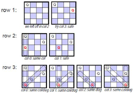
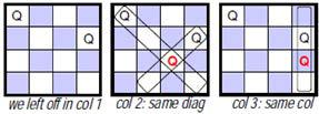
Further, backtrack to row 1, and since no columns are left, next backtrack to row 0, to obtain the final solution for 4-Queens problem as shown in Figure 1.2.10 .

Figure 1.2.10 : A final solution to the 4-Queens Problem

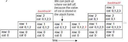
Note that finding a safe column is the core of the n-Queens solution strategy. The algorithm for finding a safe column is presented in the findSafeColumn() function below, and Figure 1.2.11 , presents a snapshot of a trace for its execution.

void findSafeColumn(int row) {
if (row == boardSize) { // base case: a solution!
solutionsFound++;
displayBoard();
if (solutionsFound >= solutionTarget)
System.exit(0);
return;}
for (int col = 0; col < boardSize; col++) {
if (isSafe(row, col)) {
placeQueen(row, col);
// Move onto the next row.
//Note applying row++/++row don’t work!!
findSafeColumn(row + 1);
// If we get here, we’ve backtracked.
removeQueen(row, col);}

Figure 1.2.11 : Tracing find safe column algorithm

The outline of algorithms for recursive backtracking and for finding a single solution are respectively presented below:

//recursive backtracking algorithm
void findSolutions(n, other-params) {
if (found a solution) {
solutionsFound++;
displaySolution();
if (solutionsFound >= solutionTarget)
System.exit(0);
return;}
for (val = first to last) {
if (isValid(val, n)) {
applyValue(val, n);
findSolutions(n + 1, other params);
removeValue(val, n);}

// finding a single solution

boolean findSolutions(n, other-params) {
if (found a solution) {
displaySolution();
return true;}
for (val = first to last) {
if (isValid(val, n)) {
applyValue(val, n);
if (findSolutions(n + 1, other params))
return true;
removeValue(val, n); }
return false;}

The data structures to support the n-Queens solution implementation are now discussed. The solution to the n-Queens problem requires three key operations:

isSafe(row, col) - check to see if a position is safe

placeQueen(row, col)

removeQueen(row, col)

Therefore, a two-dimensional array of booleans would be sufficient, as defined below:

boolean[][] queenOnSquare;

The advantage of the array data structure is the easy to implement the operations place or remove a queen, that is:

placeQueen(int row, int col) {
queenOnSquare[row][col] = true;}
removeQueen(int row, int col) {
queenOnSquare[row][col] = false;}

But then, the isSafe() operation inherently take a significant number of steps. To work around this problem additional data structures for n-Queens can facilitate improvement for the isSafe() operation. We shall add three arrays of booleans:

boolean[] colEmpty;

boolean[] upDiagEmpty;

boolean[] downDiagEmpty;

An entry in one of these arrays will true if there are no queens in the column or diagonal and false otherwise. Finally, numbering diagonals to get the indices into the arrays is done in two ways as shown in Figure 1.2.12 . In the left board of Figure 1.2.12 “upDiag = row + col” and on the right board on the figure “downDiag = (boardSize – 1) + row – col”.

Figure 1.2.12 : Numbering Diagonals

More fine tuning done using the additional arrays lead to improved isSafe()operation performance. Note that the place and remove queen operations now involve updating four arrays instead of just one as shown by the code below:

void placeQueen(int row, int col) {
queenOnSquare[row][col] = true;
colEmpty[col] = false;
upDiagEmpty[row + col] = false;
downDiagEmpty[(boardSize - 1) + row - col] = false;}

On the other hand, checking if a square is safe become more efficient, that is:

boolean isSafe(int row, int col) {
return (colEmpty[col] && upDiagEmpty[row + col] &&
downDiagEmpty[(boardSize - 1) + row - col]);}

Conclusion

This activity reviewed the key problem solving methods: iteration, recursion and recursive backtracking. The activity demonstrated use of each method using some concrete examples.

Assessment

1. Distinguish between the following problem solving methods:

1. Iteration and recursion

2. Recursion and recursive backtracking

2. Write both an iterative and recursive solution for the factorial problem.