1.3: Activity 3 - Dynamic Programming

Introduction

Dynamic Programming (DP) is about always remembering answers to the sub-problems you’ve already solved. Suppose that we have a machine, and to determine its state at time t, we have certain quantities called state variables. There will be certain times when we have to make a decision which affects the state of the system, which may or may not be known to us in advance. These decisions or changes are equivalent to transformations of state variables. The results of the previous decisions help us in choosing the future ones.

What do we conclude from this? We need to break up a problem into a series of overlapping sub-problems, and build up solutions to larger and larger sub-problems. If you are given a problem, which can be broken down into smaller sub-problems, and these smaller sub-problems can still be broken into smaller ones - and if you manage to find out that there are some over-lapping sub-problems, then you’ve encountered a DP problem.

Famous DP algorithms include:

• Unix diff for comparing two files
• Bellman-Ford for shortest path routing in networks
• TeX the ancestor of LaTeX
• WASP - Winning and Score Predictor

Activity Details

The core idea of Dynamic Programming is to avoid repeated work by remembering partial results and this concept finds application in many real life situations. In programming, DP is a powerful technique that allows one to solve different types of problems in time O(n2) or O(n3) for which a naive approach would take exponential time.

A naive illustration of what dynamic programming really is summed below:

• Writes down “1+1+1+1+1+1+1+1 =” on a sheet of paper.
• “What’s that equal to?”
• Counting “Eight!”
• Writes down another “1+” on the left.
• “What about that?”
• “Nine!” “How would you know it was nine so fast?”
• “You just added one more!”
• “So you didn’t need to recount because you remembered!

Dynamic Programming and Recursion

Dynamic programming is basically, recursion plus using common sense. What it means is that recursion allows you to express the value of a function in terms of other values of that function. Common sense tells you that if you implement a function in a way that the recursive calls are done in advance and stored for easy access it will make the program faster. This is what we call Memoization - it is memorizing the results of some specific states, which can then be later accessed to solve other sub-problems.

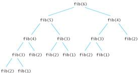
The intuition behind dynamic programming is that we trade space for time, i.e. to say that instead of calculating all the states taking a lot of time but no space, we take up space to store the results of all the sub-problems to save time later. For example, consider the following recurrent definition of Fibonacci numbers:

Fibonacci (n) = 1; if n = 0

Fibonacci (n) = 1; if n = 1

Fibonacci (n) = Fibonacci(n-1) + Fibonacci(n-2)

The first few numbers in this series are: 1, 1, 2, 3, 5, 8, 13, 21,..., and so on! Code for determining the nth number in the series using recursion is as follows:

int ibf (int n) {
    if (n < 2)
        return 1;
    return fib(n-1) + fib(n-2);}

Using Dynamic Programming approach with memorization we define the following code:

void fib () {
    fibresult[0] = 1;
    fibresult[1] = 1;
    for (int i = 2; i<n; i++) 
    fibresult[i] = fibresult[i-1] + fibresult[i-2];}

Are we using a different recurrence relation in the two codes? No. Are we doing anything different in the two codes? Yes! In the recursive code, a lot of values are being recalculated multiple times. We could do better by calculating each unique quantity only once. Consider the recursive method trace shown in Figure 1.3.1 to understand how certain values were being recalculated in the recursive way:

Figure 1.3.1 : Recursive Fibonacci trace for n=6

Most of the DP problems can be categorized into two types:

• Optimization problems
• Combinatorial problems

The optimization problems expect you to select a feasible solution, so that the value of the required function is minimized or maximized. Combinatorial problems expect you to figure out the number of ways to do something, or the probability of some event happening.

Every Dynamic Programming problem has a schema to be followed:

• Show that the problem can be broken down into optimal sub-problems
• Recursively define the value of the solution by expressing it in terms of optimal solutions for smaller sub-problems
• Compute the value of the optimal solution in bottom-up fashion
• Construct an optimal solution from the computed information

One can think of dynamic programming as a table-filling algorithm: you know the calculations you have to do, so you pick the best order to do them in and ignore the ones you don’t have to fill in. Consider the following sample problem:

Suppose you are given a number N. Find the number of different ways to write it as the sum of 1, 3 and 4. For example, if N = 5, the answer would be 6:

i.	1 + 1 + 1 + 1 + 1
ii.	1 + 4
iii.	4 + 1
iv.	1 + 1 + 3
v.	1 + 3 + 1
vi.	3 + 1 + 1

Sub-problem: Let DPn be the number of ways to write N as the sum of 1, 3, and 4.

Finding recurrence: Consider one possible solution, n = x1 + x2 + ... xn. If the last number is 1, the sum of the remaining numbers should be n - 1. So, number of sums that end with 1 is equal to DPn-1. Take other cases into account where the last number is 3 and 4. The final recurrence would be:

DPn = DPn-1 + DPn-3 + DPn-4.

Take care of the base cases: DP0 = DP1 = DP2 = 1, and DP3 = 2. The code corresponding implementation is shown below:

DP[0] = DP[1] = DP[2] = 1; DP[3] = 2;
for (i = 4; i <= n; i++) {
DP[i] = DP[i-1] + DP[i-3] + DP[i-4]; }

The above technique takes a bottom up approach and uses memoization to avoid computing results that have already been computed.

The following narrates a puzzle to aspire the power of dynamic programming solution method:

“Imagine you have a collection of N wines placed next to each other on a shelf. For simplicity, let’s number the wines from left to right as they are standing on the shelf with integers from 1 to N, respectively. Suppose the initial price of the ith wine is pi (prices of wines can be different). Because wines get better every year on year y the price of the ith wine will be y*pi, i.e. y-times the initial current year value.

Suppose we want to sell all the wines but can only sell exactly one wine per year, starting from the current year. More-over, on each year we are only allowed to sell either the leftmost or the rightmost wine on the shelf and not allowed to reorder the wines on the shelf (i.e. they must stay in the same order as they are at the beginning). What is the maximum profit obtained by selling the wines in optimal order?

For example, if the prices of the wines are (in the order as they are placed on the shelf, from left to right): p1=1, p2=4, p3=2, p4=3. The optimal solution would be to sell the wines in the order p1, p4, p3, p2 for a total profit 1 * 1 + 3 * 2 + 2 * 3 + 4 * 4 = 29.

Wrong solution!

After playing with the problem for a while, you’ll probably get the feeling, that in the optimal solution you want to sell the expensive wines as late as possible. You can probably come up with the following greedy strategy:

Every year, sell the cheaper of the two (leftmost and rightmost) available wines.

Although the strategy doesn’t mention what to do when the two wines cost the same, this strategy feels right. But unfortunately, it isn’t, as the following example demonstrates.

If the prices of the wines are: p1=2, p2=3, p3=5, p4=1, p5=4. The greedy strategy would sell them in the order p1, p2, p5, p4, p3 for a total profit 2 * 1 + 3 * 2 + 4 * 3 + 1 * 4 + 5 * 5 = 49.

But, we can do better if we sell the wines in the order p1, p5, p4, p2, p3 for a total profit 2 * 1 + 4 * 2 + 1 * 3 + 3 * 4 + 5 * 5 = 50.

This counter-example should convince you, that the problem is not so easy as it can look on a first sight and it can be solved using DP.

DP Solution using a backtrack

When coming up with the memoization solution for a problem, start with a backtrack solution that finds the correct answer. Backtrack solution enumerates all the valid answers for the problem and chooses the best one. Below are some restrictions on the backtrack solution:

• It should be a function, calculating the answer using recursion
• It should return the answer with return statement, i.e., not store it somewhere
• All the non-local variables that the function uses should be used as read-only, i.e. the function can modify only local variables and its arguments.

The following code uses the backtrack approach:

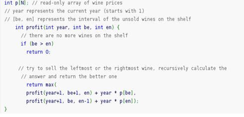
The above solution simply tries all the possible valid orders of selling the wines. If there are N wines in the beginning, it will try 2^N possibilities (each year we have 2 choices). But even though we get the correct answer, the time complexity of the algorithm grows exponentially.

The correctly written backtrack function should always represent an answer to a well-stated question. In our case profit function represents an answer to a question: “What is the best profit we can get from selling the wines with prices stored in the array p, when the current year is year and the interval of unsold wines spans through [be, en], inclusive?”. You should always try to create such a question for your backtrack function to see if you got it right and understand exactly what it does.

We should try to minimize the state space of function arguments. In this step think about, which of the arguments you pass to the function are redundant. Either we can construct them from the other arguments or we don’t need them at all. If there are any such arguments, don’t pass them to the function. Just calculate them inside the function.

In the above function profit, the argument year is redundant. It is equivalent to the number of wines we have already sold plus one, which is equivalent to the total number of wines from the beginning minus the number of wines we have not sold plus one. If we create a read-only global variable N, representing the total number of wines in the beginning, we can rewrite our function as follows:

int N; // read-only number of wines in the beginning 
int p[N]; // read-only array of wine prices
    int profit(int be, int en) {
        if (be > en)
            return 0;
        // (en-be+1) is the number of unsold wines
        int year = N - (en-be+1) + 1; // as in the description above
        return max(
            profit(be+1, en) + year * p[be],
            profit(be, en-1) + year * p[en]); }

We are now 99% done. To transform the backtrack function with time complexity O(2N) into the memoization solution with time complexity O(N2), we will use a little trick which doesn’t require almost any thinking. As noted above, there are only O(N2) different arguments our function can be called with. In other words, there are only O(N2) different things we can actually compute.

So where does O(2N) time complexity comes from and what does it compute? The answer is - the exponential time complexity comes from the repeated recursion and because of that, it computes the same values again and again. If you run the above code for an arbitrary array of N=20 wines and calculate how many times the function was called for arguments be=10 and en=10 you will get a number 92378.

That’s a huge waste of time to compute the same answer that many times. What we can do to improve this is to memoize the values once we have computed them and every time the function asks for an already memoized value, we don’t need to run the whole recursion again, as shown in the following code:

int N; // read-only number of wines in the beginning

int p[N]; // read-only array of wine prices

int cache[N][N]; // all values initialized to -1 (or anything you choose)

int profit(int be, int en) {
    if (be > en)
        return 0;
    // these two lines save the day
    if (cache[be][en] != -1)
        return cache[be][en];
    int year = N - (en-be+1) + 1;
    // when calculating the new answer, don’t forget to cache it
    return cache[be][en] = max(
        profit(be+1, en) + year * p[be],
        profit(be, en-1) + year * p[en]); }

To sum it up, if you identify that a problem can be solved using DP, try to create a backtrack function that calculates the correct answer. Try to avoid the redundant arguments, minimize the range of possible values of function arguments and also try to optimize the time complexity of one function call (remember, you can treat recursive calls as they would run in O(1) time). Finally, you can memoize the values and don’t calculate the same things twice.

Conclusion

This activity presented the dynamic programming problem solving approach. Dynamic programming is basically recursion and use of common sense to store (memoize) some recursive calls results and access the results to speed computation of other sub-problems.

Assessment

1. Explain the schema to be followed when solving a DP problem.
2. How do the DP with backtrack method differs from recursive backtracking?