10.6: Congestion

Last updated
Save as PDF

Page ID: 48361

Eric Lehman, F. Thomson Leighton, & Alberty R. Meyer
Google and Massachusetts Institute of Technology via MIT OpenCourseWare

\( \newcommand{\vecs}[1]{\overset { \scriptstyle \rightharpoonup} {\mathbf{#1}} } \) \( \newcommand{\vecd}[1]{\overset{-\!-\!\rightharpoonup}{\vphantom{a}\smash {#1}}} \)\(\newcommand{\id}{\mathrm{id}}\) \( \newcommand{\Span}{\mathrm{span}}\) \( \newcommand{\kernel}{\mathrm{null}\,}\) \( \newcommand{\range}{\mathrm{range}\,}\) \( \newcommand{\RealPart}{\mathrm{Re}}\) \( \newcommand{\ImaginaryPart}{\mathrm{Im}}\) \( \newcommand{\Argument}{\mathrm{Arg}}\) \( \newcommand{\norm}[1]{\| #1 \|}\) \( \newcommand{\inner}[2]{\langle #1, #2 \rangle}\) \( \newcommand{\Span}{\mathrm{span}}\) \(\newcommand{\id}{\mathrm{id}}\) \( \newcommand{\Span}{\mathrm{span}}\) \( \newcommand{\kernel}{\mathrm{null}\,}\) \( \newcommand{\range}{\mathrm{range}\,}\) \( \newcommand{\RealPart}{\mathrm{Re}}\) \( \newcommand{\ImaginaryPart}{\mathrm{Im}}\) \( \newcommand{\Argument}{\mathrm{Arg}}\) \( \newcommand{\norm}[1]{\| #1 \|}\) \( \newcommand{\inner}[2]{\langle #1, #2 \rangle}\) \( \newcommand{\Span}{\mathrm{span}}\)\(\newcommand{\AA}{\unicode[.8,0]{x212B}}\)

The complete binary tree has a fatal drawback: the root switch is a bottleneck. At best, this switch must handle right and vice-versa. Passing all these packets through a single switch could take a long time. At worst, if this switch fails, the network is broken into two equal-sized pieces.

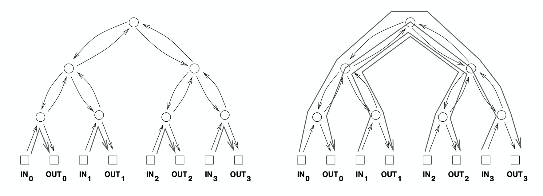
It’s true that if the routing problem is given by the identity permutation, \(Id(i) ::= i\), then there is an easy routing, \(P\), that solves the problem: let \(P_i\) be the path from input \(i\) up through one switch and back down to output \(i\). On the other hand, if the problem was given by \(\pi(i) ::= (N-1) - i\), then in any solution, \(Q\), for \(\pi\), each path \(Q_i\) beginning at input \(i\) must eventually loop all the way up through the root switch and then travel back down to output \((N-1) - i\). These two situations are illustrated below. We can distinguish between a “good” set of paths and a “bad” set based on congestion. The congestion of a routing, \(P\), is equal to the largest number of paths in \(P\) that pass through a single switch. For example, the congestion of the routing on the left is 1, since at most 1 path passes through each switch. However, the congestion of the routing on the right is 4, since 4 paths pass through the root switch (and the two switches directly below the root). Generally, lower congestion is better since packets can be delayed at an overloaded switch.

By extending the notion of congestion to networks, we can also distinguish between “good” and “bad” networks with respect to bottleneck problems. For each routing problem, \(\pi\), for the network, we assume a routing is chosen that optimizes congestion, that is, that has the minimum congestion among all routings that solve \(\pi\). Then the largest congestion that will ever be suffered by a switch will be the maximum congestion among these optimal routings. This “maximin” congestion is called the congestion of the network.

So for the complete binary tree, the worst permutation would be \(\pi(i) ::= (N-1)-i\). Then in every possible solution for \(\pi\), every packet would have to follow a path passing through the root switch. Thus, the max congestion of the complete binary tree is \(N\)—which is horrible!

Let’s tally the results of our analysis so far: