10.8: Butterfly

The Holy Grail of switching networks would combine the best properties of the complete binary tree (low diameter, few switches) and of the array (low congestion). The butterfly is a widely-used compromise between the two.

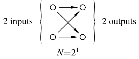
A good way to understand butterfly networks is as a recursive data type. The recursive definition works better if we define just the switches and their connections, omitting the terminals. So we recursively define \(F_n\) to be the switches and connections of the butterfly net with \(N ::= 2^n\) input and output switches.

The base case is \(F_1\) with 2 input switches and 2 output switches connected as in Figure 10.1.

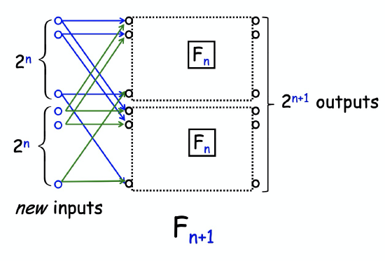
In the constructor step, we construct \(F_{n+1}\) with \(2^{n+1}\) inputs and outputs out of two \(F_n\) nets connected to a new set of \(2^{n+1}\) input switches, as shown in as in Figure 10.2. That is, the \(i\)th and \(2^n + i\)th new input switches are each connected to the same two switches, the \(i\)th input switches of each of two \(F_n\) components for \(i = 1, \ldots, 2^n\). The output switches of \(F_{n+1}\) are simply the output switches of each of the \(F_n\) copies.

Figure 10.1 \(F_1\), the Butterfly Net switches with \(N = 2^1\).

So \(F_{n+1}\) is laid out in columns of height \(2^{n+1}\) by adding one more column of switches to the columns in \(F_n\). Since the construction starts with two columns when \(n + 1\), the \(F_{n+1}\) switches are arrayed in \(n + 1\) columns. The total number of switches is the height of the columns times the number of columns, \(2^{n+1} (n+1)\). Remembering that \(n = \log N\), we conclude that the Butterfly Net with \(N\) inputs has \(N (\log N + 1)\) switches.

Since every path in \(F_{n+1}\) from an input switch to an output is the same length, \(n + 1\), the diameter of the Butterfly net with \(2^{n+1}\) inputs is this length plus two because of the two edges connecting to the terminals (square boxes) —one edge from input terminal to input switch (circle) and one from output switch to output terminal.

There is an easy recursive procedure to route a packet through the Butterfly Net. In the base case, there is only one way to route a packet from one of the two inputs to one of the two outputs. Now suppose we want to route a packet from an input switch to an output switch in \(F_{n+1}\). If the output switch is in the “top” copy of \(F_{n}\), then the first step in the route must be from the input switch to the unique switch it is connected to in the top copy; the rest of the route is determined by recursively routing the rest of the way in the top copy of \(F_{n}\). Likewise, if the output switch is in the “bottom” copy of \(F_{n}\), then the first step in the route must be to the switch in the bottom copy, and the rest of the route is determined by recursively routing in the bottom copy of \(F_{n}\). In fact, this argument shows that the routing is unique: there is exactly one path in the Butterfly Net from each input to each output, which implies that the network latency when minimizing congestion is the same the diameter.

The congestion of the butterfly network is about p as \(\sqrt{N}\). More precisely, the congestion is \(\sqrt{N}\) if \(N\) is an even power of 2 and \(\sqrt{N/2}\) if \(N\) is an odd power of 2. A simple proof of this appears in Problem 10.8.

Figure 10.2 \(F_{n+1}\), the Butterfly Net switches with \(2^{n+1}\) inputs and outputs.

Let’s add the butterfly data to our comparison table:

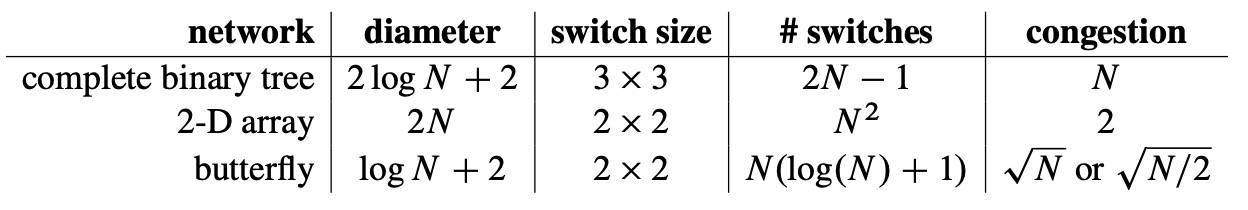
The butterfly has lower congestion than the complete binary tree. It also uses fewer switches and has lower diameter than the array. However, the butterfly does not capture the best qualities of each network, but rather is a compromise somewhere between the two. Our quest for the Holy Grail of routing networks goes on.