11.9: Connectivity

Definition \(\PageIndex{1}\)

Two vertices are connected in a graph when there is a path that begins at one and ends at the other. By convention, every vertex is connected to itself by a path of length zero. A graph is connected when every pair of vertices are connected.

Connected Components

Being connected is usually a good property for a graph to have. For example, it could mean that it is possible to get from any node to any other node, or that it is possible to communicate between any pair of nodes, depending on the application.

But not all graphs are connected. For example, the graph where nodes represent cities and edges represent highways might be connected for North American cities, but would surely not be connected if you also included cities in Australia. The same is true for communication networks like the internet—in order to be protected from viruses that spread on the internet, some government networks are completely isolated from the internet.

Figure 11.16 One graph with 3 connected components.

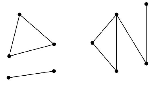
Another example is shown in Figure 11.16, which looks like a picture of three graphs, but is intended to be a picture of one graph. This graph consists of three pieces (subgraphs). Each piece by itself is connected, but there are no paths between vertices in different pieces. These connected pieces of a graph are called its connected components.

Definition \(\PageIndex{2}\)

A connected component of a graph is a subgraph consisting of some vertex and every node and edge that is connected to that vertex.

So, a graph is connected iff it has exactly one connected component. At the other extreme, the empty graph on \(n\) vertices has \(n\) connected components.

Odd Cycles and 2-Colorability

We have already seen that determining the chromatic number of a graph is a challenging problem. There is one special case where this problem is very easy, namely, when the graph is 2-colorable

Theorem \(\PageIndex{3}\)

The following graph properties are equivalent:

1. The graph contains an odd length cycle.
2. The graph is not 2-colorable.
3. The graph contains an odd length closed walk.

In other words, if a graph has any one of the three properties above, then it has all of the properties.

We will show the following implications among these properties:

1. IMPLIES 2. IMPLIES 3. IMPLIES 1:

So each of these properties implies the other two, which means they all are equivalent.

1 IMPLIES 2 Proof. This follows from equation 11.7.1. \(\quad \blacksquare\)

2 IMPLIES 3 If we prove this implication for connected graphs, then it will hold for an arbitrary graph because it will hold for each connected component. So we can assume that \(G\) is connected.

Proof. Pick an arbitrary vertex \(r\) of \(G\). Since \(G\) is connected, for every node \(u \in V(G)\), there will be a walk \(\textbf{w}_u\) starting at \(u\) and ending at \(r\). Assign colors to vertices of \(G\) as follows:

\[ \nonumber \text{color}(u) = \left\{\begin{array}{ll} \text{black}, & \text { if } |\textbf{w}_u| \text { is even,} \\ \text{white}, & \text { otherwise. } \end{array}\right.\]

Now since \(G\) is not colorable, this can’t be a valid coloring. So there must be an edge between two nodes \(u\) and \(v\) with the same color. But in that case

\[\nonumber \textbf{w}_u \hat{} \text{reverse}(\textbf{w}_u) \hat{} \langle v - u \rangle\]

is a closed walk starting and ending at \(u\), and its length is

\[\nonumber |\textbf{w}_u| + |\textbf{w}_v| + 1\]

which is odd. \(\quad \blacksquare\)

3 IMPLIES 1 Proof. Since there is an odd length closed walk, the WOP implies there is an odd length closed walk \(w\) of minimum length. We claim \(w\) must be a cycle. To show this, assume to the contrary that \(w\) is not a cycle, so there is a repeat vertex occurrence besides the start and end. There are then two cases to consider depending on whether the additional repeat is different from, or the same as, the start vertex.

In the first case, the start vertex has an extra occurrence. That is,

\[\nonumber \textbf{w} = \textbf{f} \hat{x} \textbf{r}\]

for some positive length walks \(\textbf{f}\) and \(\textbf{r}\) that begin and end at \(x\). Since

\[\nonumber |\textbf{w}| = |\textbf{f}| + |\textbf{r}|\]

is odd, exactly one of \(\textbf{f}\) and \(\textbf{r}\) must have odd length, and that one will be an odd length closed walk shorter than \(\textbf{w}\), a contradiction.

In the second case,

\[\nonumber \textbf{w} = \textbf{f} \hat{y} \textbf{g} \hat{y} \textbf{r}\]

where \(\textbf{f}\) is a walk from \(x\) to \(y\) for some \(y \neq x\), and \(\textbf{r}\) is a walk from \(y\) to \(x\), and \(|\textbf{g}| > 0\). Now \(\textbf{g}\) cannot have odd length or it would be an odd-length closed walk shorter than \(\textbf{w}\). So \(\textbf{g}\) has even length. That implies that \(\textbf{f} \hat{y} \textbf{r}\) must be an odd-length closed walk shorter than \(w\), again a contradiction.

This completes the proof of Theorem 11.9.3. \(\quad \blacksquare\)

Theorem 11.9.3 turns out to be useful, since bipartite graphs come up fairly often in practice. We’ll see examples when we talk about planar graphs in Chapter 12.

k-connected Graphs

If we think of a graph as modeling cables in a telephone network, or oil pipelines, or electrical power lines, then we not only want connectivity, but we want connectivity that survives component failure. So more generally, we want to define how strongly two vertices are connected. One measure of connection strength is how many links must fail before connectedness fails. In particular, two vertices are \(k\)-edge connected when it takes at least \(k\) “edge-failures” to disconnect them. More precisely:

Definition \(\PageIndex{4}\)

Two vertices in a graph are \(k\)-edge connected when they remain connected in every subgraph obtained by deleting up to \(k - 1\) edges. A graph is \(k\)-edge connected when it has more than one vertex, and pair of distinct vertices in the graph are \(k\)-connected.

Notice that according to Definition 11.9.4, if a graph is \(k\)-connected, it is also \(j\)-connected for \(j \leq k\). This convenient convention implies that two vertices are connected according to definition 11.9.1 iff they are 1-edge connected according to Definition 11.9.4. From now on we’ll drop the “edge” modifier and just say “\(k\)-connected.”⁹

For example, in the graph in figure 11.15, vertices \(c\) and \(e\) are 3-connected, \(b\) and \(e\) are 2-connected, \(g\) and \(e\) are 1 connected, and no vertices are 4-connected. The graph as a whole is only 1-connected. A complete graph, \(k_n\), is \(n-1\)- connected. Every cycle is 2-connected.

The idea of a cut edge is a useful way to explain 2-connectivity.

Definition \(\PageIndex{5}\)

If two vertices are connected in a graph \(G\), but not connected when an edge \(e\) is removed, then \(e\) is called a cut edge of \(G\).

So a graph with more than one vertex is 2-connected iff it is connected and has no cut edges. The following Lemma is another immediate consequence of the definition:

Lemma 11.9.6. An edge is a cut edge iff it is not on a cycle.

More generally, if two vertices are connected by \(k\) edge-disjoint paths—that is, no edge occurs in two paths—then they must be \(k\)-connected, since at least one edge will have to be removed from each of the paths before they could disconnect. A fundamental fact, whose ingenious proof we omit, is Menger’s theorem which confirms that the converse is also true: if two vertices are \(k\)-connected, then there are \(k\) edge-disjoint paths connecting them. It takes some ingenuity to prove this just for the case \(k = 2\).

The Minimum Number of Edges in a Connected Graph

The following theorem says that a graph with few edges must have many connected components.

Theorem \(\PageIndex{7}\)

Every graph, \(G\), has at least \(|V(G)| - |E(G)|\) connected components.

Of course for Theorem 11.9.7 to be of any use, there must be fewer edges than vertices.

Proof

We use induction on the number, \(k\), of edges. Let \(P(k)\) be the proposition that

every graph, \(G\), with \(k\) edges has at least \(|V(G)|-k\) connected components.

Base case (\(k = 0\)): In a graph with 0 edges, each vertex is itself a connected component, and so there are exactly \(|V(G)|=|V(G)| - 0\) connected components. So \(P(0)\) holds.

Inductive step: Let \(G_e\) be the graph that results from removing an edge, \(e\ in E(G)\). So \(G_e\) has \(k\) edges, and by the induction hypothesis \(P(k)\), we may assume that \(G_e\) has at least \(|V(G)-k|\)-connected components. Now add back the edge \(e\) to obtain the original graph \(G\). If the endpoints of \(e\) were in the same connected component of \(G_e\), then \(G\) has the same sets of connected vertices as \(G_e\), so \(G\) has at least \(|V(G)| - k > |V(G)| - (k+1)\) components. Alternatively, if the endpoints of \(e\) were in different connected components of \(G_e\), then these two components are merged into one component in \(G\), while all other components remain unchanged, so that \(G\) has one fewer connected component than \(G_e\). That is, \(G\) has at least \((|V(G)| - k) - 1> |V(G)| - (k+1)\) connected components. So in either case, \(G\) has at least \(|V(G)| - (k+1)\) components, as claimed.

This completes the inductive step and hence the entire proof by induction. \(\quad \blacksqure\)

Corollary 11.9.8. Every connected graph with \(n\) vertices has at least \(n - 1\) edges.

A couple of points about the proof of Theorem 11.9.7 are worth noticing. First, we used induction on the number of edges in the graph. This is very common in proofs involving graphs, as is induction on the number of vertices. When you’re presented with a graph problem, these two approaches should be among the first you consider.

The second point is more subtle. Notice that in the inductive step, we took an arbitrary \((k+1)\)-edge graph, threw out an edge so that we could apply the induction assumption, and then put the edge back. You’ll see this shrink-down, grow-back process very often in the inductive steps of proofs related to graphs. This might seem like needless effort: why not start with an \(k\)-edge graph and add one more to get an \((k+1)\)-edge graph? That would work fine in this case, but opens the door to a nasty logical error called buildup error, illustrated in Problem 11.48.

⁹There is a corresponding definition of \(k\)-vertex connectedness based on deleting vertices rather than edges. Graph theory texts usually use “\(k\)-connected” as shorthand for “\(k\)-vertex connected.” But edge-connectedness will be enough for us.