2.3: Measures of Reliability and Failure Tolerance

Availability and Mean Time to Failure

A useful model of a system or a system component, from a reliability point of view, is that it operates correctly for some period of time and then it fails. The time to failure (TTF) is thus a measure of interest, and it is something that we would like to be able to predict. If a higher-level module does not mask the failure and the failure is persistent, the system cannot be used until it is repaired, perhaps by replacing the failed component, so we are equally interested in the time to repair (TTR). If we observe a system through \(N\) run–fail–repair cycles and observe in each cycle \(i\) the values of \(TTF_i\) and \(TTR_i\), we can calculate the fraction of time it operated properly, a useful measure known as availability:

\[ Availability = \frac{\text{time system was running}}{\text{time system should have been running}} = \dfrac{\displaystyle \sum_{i=1}^N TTF_i}{\displaystyle \sum_{i=1}^N (TTF_i + TTR_i)} \]

By separating the denominator of the availability expression into two sums and dividing each by \(N\) (the number of observed failures) we obtain two time averages that are frequently reported as operational statistics: the mean time to failure (MTTF) and the mean time to repair (MTTR):

\[ MTTF = \frac{1}{N} \sum_{i=1}^N TTF _i \quad\quad MTTR = \frac{1}{N} \sum_{i=1}^N TTR _i \]

The sum of these two statistics is usually called the mean time between failures (MTBF). Thus availability can be variously described as

\[ Availability = \frac{MTTF}{MTBF} = \frac{MTTF}{MTTF + MTTR} = \frac{MTBF - MTTR}{MTBF} \]

In some situations, it is more useful to measure the fraction of time that the system is not working, known as its down time:

\[ \text{Down time} = (1 - Availability) = \frac{MTTR}{MTBF} \]

One thing that the definition of down time makes clear is that MTTR and MTBF are, in some sense, equally important. One can reduce down time either by reducing MTTR or by increasing MTBF.

Components are often repaired by simply replacing them with new ones. When failed components are discarded rather than fixed and returned to service, it is common to use a slightly different method to measure MTTF. The method is to place a batch of \(N\) components in service in different systems (or in what is hoped to be an equivalent test environment), run them until they have all failed, and use the set of failure times as the \(TTF_i\) in Equation \(\PageIndex{2}\). This procedure substitutes an ensemble average for the time average. We could use this same procedure on components that are not usually discarded when they fail, in the hope of determining their MTTF more quickly, but we might obtain a different value for the MTTF. Some failure processes do have the property that the ensemble average is the same as the time average (processes with this property are called ergodic), but other failure processes do not. For example, the repair itself may cause wear, tear, and disruption to other parts of the system, in which case each successive system failure might on average occur sooner than did the previous one. If that is the case, an MTTF calculated from an ensemble-average measurement might be too optimistic.

As we have defined them, availability, MTTF, MTTR, and MTBF are backward-looking measures. They are used for two distinct purposes: (1) for evaluating how the system is doing (compared, for example, with predictions made when the system was designed) and (2) for predicting how the system will behave in the future. The first purpose is concrete and well defined. The second requires that one take on faith that samples from the past provide an adequate predictor of the future, which can be a risky assumption. There are other problems associated with these measures. While MTTR can usually be measured in the field, the more reliable a component or system the longer it takes to evaluate its MTTF, so that measure is often not directly available. Instead, it is common to use and measure proxies to estimate its value. The quality of the resulting estimate of availability then depends on the quality of the proxy.

A typical 3.5-inch magnetic disk comes with a reliability specification of 300,000 hours "MTTF", which is about 34 years. Since the company quoting this number has probably not been in business that long, it is apparent that whatever they are calling "MTTF" is not the same as either the time-average or the ensemble-average MTTF that we just defined. It is actually a quite different statistic, which is why we put quotes around its name. Sometimes this "MTTF" is a theoretical prediction obtained by modeling the ways that the components of the disk might be expected to fail and calculating an expected time to failure.

A more likely possibility is that the manufacturer measured this "MTTF" by running an array of disks simultaneously for a much shorter time and counting the number of failures. For example, suppose the manufacturer ran 1,000 disks for 3,000 hours (about four months) each, and during that time 10 of the disks failed. The observed failure rate of this sample is 1 failure for every 300,000 hours of operation. The next step is to invert the failure rate to obtain 300,000 hours of operation per failure and then quote this number as the "MTTF". But the relation between this sample observation of failure rate and the real MTTF is problematic. If the failure process were memoryless (meaning that the failure rate is independent of time; Section 2.3.2, below, explores this idea more thoroughly), we would have the special case in which the MTTF really is the inverse of the failure rate. A good clue that the disk failure process is not memoryless is that the disk specification may also mention an "expected operational lifetime" of only 5 years. That statistic is probably the real MTTF—though even that may be a prediction based on modeling rather than a measured ensemble average. An appropriate re-interpretation of the 34-year "MTTF" statistic is to invert it and identify the result as a short-term failure rate that applies only within the expected operational lifetime. The paragraph discussing Equation \(\PageIndex{9}\) in Section 2.3.2, describes a fallacy that sometimes leads to miscalculation of statistics such as the MTTF.

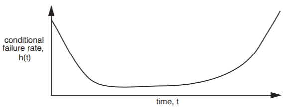
Magnetic disks, light bulbs, and many other components exhibit a time-varying statistical failure rate known as a bathtub curve, illustrated in Figure \(\PageIndex{1}\) and defined more carefully in Section 2.3.2, below. When components come off the production line, a certain fraction fail almost immediately because of gross manufacturing defects. Those components that survive this initial period usually run for a long time with a relatively uniform failure rate. Eventually, accumulated wear and tear cause the failure rate to increase again, often quite rapidly, producing a failure rate plot that resembles the shape of a bathtub.

Figure \(\PageIndex{1}\): A bathtub curve, showing how the conditional failure rate of a component changes with time.

Several other suggestive and colorful terms describe these phenomena. Components that fail early are said to be subject to infant mortality, and those that fail near the end of their expected lifetimes are said to burn out. Manufacturers sometimes burn in such components by running them for a while before shipping, with the intent of identifying and discarding the ones that would otherwise fail immediately upon being placed in service. When a vendor quotes an "expected operational lifetime," it is probably the mean time to failure of those components that survive burn in, while the much larger "MTTF" number is probably the inverse of the observed failure rate at the lowest point of the bathtub. (The published numbers also sometimes depend on the outcome of a debate between the legal department and the marketing department, but that gets us into a different topic.) A chip manufacturer describes the fraction of components that survive the burn-in period as the yield of the production line. Component manufacturers usually exhibit a phenomenon known informally as a learning curve, which simply means that the first components coming out of a new production line tend to have more failures than later ones. The reason is that manufacturers design for iteration: upon seeing and analyzing failures in the early production batches, the production line designer figures out how to refine the manufacturing process to reduce the infant mortality rate.

One job of the system designer is to exploit the nonuniform failure rates predicted by the bathtub and learning curves. For example, a conservative designer exploits the learning curve by avoiding the latest generation of hard disks in favor of slightly older designs that have accumulated more field experience. One can usually rely on other designers who may be concerned more about cost or performance than availability to shake out the bugs in the newest generation of disks.

The 34-year "MTTF" disk drive specification may seem like public relations puffery in the face of the specification of a 5-year expected operational lifetime, but these two numbers actually are useful as a measure of the nonuniformity of the failure rate. This nonuniformity is also susceptible to exploitation, depending on the operation plan. If the operation plan puts the component in a system such as a satellite, in which it will run until it fails, the designer would base system availability and reliability estimates on the 5-year figure. On the other hand, the designer of a ground-based storage system, mindful that the 5-year operational lifetime identifies the point where the conditional failure rate starts to climb rapidly at the far end of the bathtub curve, might include a plan to replace perfectly good hard disks before burn-out begins to dominate the failure rate—in this case, perhaps every 3 years. Since one can arrange to do scheduled replacement at convenient times—for example, when the system is down for another reason, or perhaps even without bringing the system down—the designer can minimize the effect on system availability. The manufacturer’s 34-year "MTTF", which is probably the inverse of the observed failure rate at the lowest point of the bathtub curve, can then be used as an estimate of the expected rate of unplanned replacements, although experience suggests that this specification may be a bit optimistic. Scheduled replacements are an example of preventive maintenance, which is active intervention intended to increase the mean time to failure of a module or system and thus improve availability. 

For some components, observed failure rates are so low that MTTF is estimated by accelerated aging. This technique involves making an educated guess about what the dominant underlying cause of failure will be and then amplifying that cause. For example, it is conjectured that failures in recordable Compact Disks are heat-related. A typical test scenario is to store batches of recorded CDs at various elevated temperatures for several months, periodically bringing them out to test them and count how many have failed. One then plots these failure rates versus temperature and extrapolates to estimate what the failure rate would have been at room temperature. Again making the assumption that the failure process is memoryless, that failure rate is then inverted to produce an MTTF. Published MTTFs of 100 years or more have been obtained this way. If the dominant fault mechanism turns out to be something else (such as bacteria munching on the plastic coating) or if after 50 years the failure process turns out not to be memoryless after all, an estimate from an accelerated aging study may be far wide of the mark. A designer must use such estimates with caution and understanding of the assumptions that went into them.

Availability is sometimes discussed by counting the number of nines in the numerical representation of the availability measure. Thus a system that is up and running 99.9% of the time is said to have 3-nines availability. Measuring by nines is often used in marketing because it sounds impressive. A more meaningful number is usually obtained by calculating the corresponding down time. A 3-nines system can be down nearly 1.5 minutes per day or 8 hours per year, a 5-nines system 5 minutes per year, and a 7-nines system only 3 seconds per year. Another problem with measuring by nines is that it only provides information about availability, not about MTTF. One 3-nines system may have a brief failure every day, while a different 3-nines system may have a single eight-hour outage once a year. Depending on the application, the difference between those two systems could be important. Any single measure should always be suspect.

Finally, availability can be a more fine-grained concept. Some systems are designed so that when they fail, some functions (for example, the ability to read data) remain available, while others (the ability to make changes to the data) are not. Systems that continue to provide partial service in the face of failure are called fail-soft, a concept defined more carefully in Section 2.4.

 

Reliability Functions

The bathtub curve expresses the conditional failure rate \(h(t)\) of a module, defined to be the probability that the module fails between time \(t\) and time \(t + dt\), given that the component is still working at time \(t\). The conditional failure rate is only one of several closely related ways of describing the failure characteristics of a component, module, or system. The \(reliability\), \(R\), of a module is defined to be 

\[ R(t) = Pr ( \text{the module has not yet failed at time \(t\), given that the module was operating at time 0} ) \]

and the unconditional failure rate \(f(t)\) is defined to be

\[ f(t) = Pr ( \text{module fails between \(t\) and \(t + dt\)} ) \]

(The bathtub curve and these two reliability functions are three ways of presenting the same information. If you are rusty on probability, a brief reminder of how they are related appears in Sidebar \(\PageIndex{1}\)) Once \(f(t)\) is at hand, one can directly calculate the MTTF: 

\[ MTTF = \int\limits_{0}^{\infty} t \cdot f(t) \ dt \]

One must keep in mind that this MTTF is predicted from the failure rate function \(f(t)\), in contrast to the MTTF of Equation \(\PageIndex{2}\), which is the result of a field measurement. The two MTTFs will be the same only if the failure model embodied in \(f(t)\) is accurate.

Sidebar \(\PageIndex{1}\)

Reliability functions

The failure rate function, the reliability function, and the bathtub curve (which in probability texts is called the conditional failure rate function, and which in operations research texts is called the hazard function) are actually three mathematically related ways of describing the same information. The failure rate function, \(f(t)\) as defined in Equation \(\PageIndex{6}\), is a probability density function, which is everywhere non-negative and whose integral over all time is 1. Integrating the failure rate function from the time the component was created (conventionally taken to be \(t = 0\)) to the present time yields 

\[ F(t) = \int\limits_0^t f(t) \ dt \nonumber \]

\(F(t)\) is the cumulative probability that the component has failed by time \(t\). The cumulative probability that the component has not failed is the probability that it is still operating at time \(t\) given that it was operating at time \(0\), which is exactly the definition of the reliability function, \(R(t)\). That is,

\[ R(t) = 1 - F(t) \nonumber \]

The bathtub curve of Figure \(\PageIndex{1}\) reports the conditional probability \(h(t)\) that a failure occurs between \(t\) and \(t + dt\), given that the component was operating at time \(t\). By the definition of conditional probability, the conditional failure rate function is thus

\[ h(t) = \frac{f(t)}{R(t)} \nonumber \]

Some components exhibit relatively uniform failure rates, at least for the lifetime of the system of which they are a part. For these components the conditional failure rate, rather than resembling a bathtub, is a straight horizontal line, and the reliability function becomes a simple declining exponential:

\[ R(t) = e^{- \left( \frac{t}{MTTF} \right)} \]

This reliability function is said to be memoryless, which simply means that the conditional failure rate is independent of how long the component has been operating. Memoryless failure processes have the nice property that the conditional failure rate is the inverse of the MTTF.

Unfortunately, as we saw in the case of the disks with the 34-year "MTTF", this property is sometimes misappropriated to quote an MTTF for a component whose conditional failure rate does change with time. This misappropriation starts with a fallacy: an assumption that the MTTF, as defined in Equation \(\PageIndex{7}\), can be calculated by inverting the measured failure rate. The fallacy arises because in general, 

\[ E (1/t) \neq 1 / E(t) \]

That is, the expected value of the inverse is not equal to the inverse of the expected value, except in certain special cases. The important special case in which they are equal is the memoryless distribution of Equation \(\PageIndex{8}\). When a random process is memoryless, calculations and measurements are so much simpler that designers sometimes forget that the same simplicity does not apply everywhere.

Just as availability is sometimes expressed in an oversimplified way by counting the number of nines in its numerical representation, reliability in component manufacturing is sometimes expressed in an oversimplified way by counting standard deviations in the observed distribution of some component parameter, such as the maximum propagation time of a gate. The usual symbol for standard deviation is the Greek letter \(\sigma\) (sigma), and a normal distribution has a standard deviation of 1.0, so saying that a component has "4.5 \(\sigma\) reliability" is a shorthand way of saying that the production line controls variations in that parameter well enough that the specified tolerance is 4.5 standard deviations away from the mean value, as illustrated in Figure \(\PageIndex{2}\). Suppose, for example, that a production line is manufacturing gates that are specified to have a mean propagation time of 10 nanoseconds and a maximum propagation time of 11.8 nanoseconds with 4.5 \(\sigma\) reliability. The difference between the mean and the maximum, 1.8 nanoseconds, is the tolerance. For that tolerance to be 4.5 \(\sigma\), \(\sigma\) would have to be no more than 0.4 nanoseconds. To meet the specification, the production line designer would measure the actual propagation times of production line samples and, if the observed variance is greater than 0.4 ns, look for ways to reduce the variance to that level.

Figure \(\PageIndex{2}\): The normal probability density function applied to production of gates that are specified to have mean propagation time of 10 nanoseconds and maximum propagation time of 11.8 nanoseconds. The upper numbers on the horizontal axis measure the distance from the mean in units of the standard deviation, \(\sigma\). The lower numbers depict the corresponding propagation times. The integral of the tail from 4.5 \(\sigma\) to \(\infty\) is so small that it is not visible in this figure.

Another way of interpreting "4.5 \(\sigma\) reliability" is to calculate the expected fraction of components that are outside the specified tolerance. That fraction is the integral of one tail of the normal distribution from 4.5 \(\sigma\) to \(\infty\), which is about 3.4 \(\times\) 10^-6 , so in our example no more than 3.4 out of each million gates manufactured would have delays greater than 11.8 nanoseconds. Unfortunately, this measure describes only the failure rate of the production line; it does not say anything about the failure rate of the component after it is installed in a system.

A currently popular quality control method, known as "Six Sigma", is an application of two of our design principles to the manufacturing process. The idea is to use measurement, feedback, and iteration (design for iteration: "you won't get it right the first time") to reduce the variance (the robustness principle: "be strict on outputs") of production-line manufacturing. The "Six Sigma" label is somewhat misleading because in the application of the method, the number 6 is allocated to deal with two quite different effects. The method sets a target of controlling the production line variance to the level of 4.5 \(\sigma\), just as in the gate example of Figure \(\PageIndex{2}\). The remaining 1.5 \(\sigma\) is the amount that the mean output value is allowed to drift away from its original specification over the life of the production line. So even though the production line may start 6 \(\sigma\) away from the tolerance limit, after it has been operating for a while one may find that the failure rate has drifted upward to the same 3.4 in a million calculated for the 4.5 \(\sigma\) case.

In manufacturing quality control literature, these applications of the two design principles are known as Taguchi methods, after their popularizer, Genichi Taguchi.

 

Measuring Fault Tolerance

It is sometimes useful to have a quantitative measure of the fault tolerance of a system. One common measure, sometimes called the failure tolerance, is the number of failures of its components that a system can tolerate without itself failing. Although this label could be ambiguous, it is usually clear from context that a measure is being discussed. Thus a memory system that includes single-error correction (Section 2.5 describes how error correction works) has a failure tolerance of one bit.

When a failure occurs, the remaining failure tolerance of the system goes down. The remaining failure tolerance is an important thing to monitor during operation of the system because it shows how close the system as a whole is to failure. One of the most common system design mistakes is to add fault tolerance but not include any monitoring to see how much of the fault tolerance has been used up, thus ignoring the safety margin principle. When systems that are nominally fault-tolerant do fail, later analysis invariably discloses that there were several failures that the system successfully masked but that somehow were never reported and thus were never repaired. Eventually, the total number of failures exceeded the designed failure tolerance of the system.

Failure tolerance is actually a single number in only the simplest situations. Sometimes it is better described as a vector, or even as a matrix showing the specific combinations of different kinds of failures that the system is designed to tolerate. For example, an electric power company might say that it can tolerate the failure of up to 15% of its generating capacity, at the same time as the downing of up to two of its main transmission lines.