2.5: Systematically Applying Redundancy

The designer of an analog system typically masks small errors by specifying design tolerances known as margins, which are amounts by which the specification is better than necessary for correct operation under normal conditions. In contrast, the designer of a digital system both detects and masks errors of all kinds by adding redundancy, either in time or in space. When an error is thought to be transient, as when a packet is lost in a data communication network, one method of masking is to resend it, an example of redundancy in time. When an error is likely to be persistent, as in a failure in reading bits from the surface of a disk, the usual method of masking is with spatial redundancy, having another component provide another copy of the information or control signal. Redundancy can be applied either in cleverly small quantities or by brute force, and both techniques may be used in different parts of the same system.

Coding: Incremental Redundancy

The most common form of incremental redundancy, known as forward error correction, consists of clever coding of data values. With data that has not been encoded to tolerate errors, a change in the value of one bit may transform one legitimate data value into another legitimate data value. Encoding for errors involves choosing as the representation of legitimate data values only some of the total number of possible bit patterns, being careful that the patterns chosen for legitimate data values all have the property that to transform any one of them to any other, more than one bit must change. The smallest number of bits that must change to transform one legitimate pattern into another is known as the Hamming distance between those two patterns. The Hamming distance is named after Richard Hamming, who first investigated this class of codes. Thus the patterns

100101

000111

have a Hamming distance of 2 because the upper pattern can be transformed into the lower pattern by flipping the values of two bits, the first bit and the fifth bit. Data fields that have not been coded for errors might have a Hamming distance as small as 1. Codes that can detect or correct errors have a minimum Hamming distance between any two legitimate data patterns of 2 or more. The Hamming distance of a code is the minimum Hamming distance between any pair of legitimate patterns of the code. One can calculate the Hamming distance between two patterns, A and B, by counting the number of ONES in \(A \oplus B\), where \(\oplus\) is the exclusive OR (XOR) operator.

Suppose we create an encoding in which the Hamming distance between every pair of legitimate data patterns is 2. Then, if one bit changes accidentally, since no legitimate data item can have that pattern, we can detect that something went wrong. However, it is not possible to figure out what the original data pattern was. If the two patterns above were two members of the code and the first bit of the upper pattern were flipped from ONE to ZERO, there is no way to tell that the result, 000101, is not the result of flipping the fifth bit of the lower pattern.

Next, suppose that we instead create an encoding in which the Hamming distance of the code is 3 or more. Here are two patterns from such a code; bits 1, 2, and 5 are different:

100101

010111

Now, a one-bit change will always transform a legitimate data pattern into an incorrect data pattern that is still at least 2 bits distant from any other legitimate pattern but only 1 bit distant from the original pattern. A decoder that receives a pattern with a one-bit error can inspect the Hamming distances between the received pattern and nearby legitimate patterns and, by choosing the nearest legitimate pattern, correct the error. If 2 bits change, this error-correction procedure will still identify a corrected data value, but it will choose the wrong one. If we expect 2-bit errors to happen often, we could choose the code patterns so that the Hamming distance is 4, in which case the code can correct 1-bit errors and detect 2-bit errors. But a 3-bit error would look just like a 1-bit error in some other code pattern, so it would decode to a wrong value. More generally, if the Hamming distance of a code is \(d\), a little analysis reveals that one can detect \(d-1\) errors and correct \(\lfloor (d - 1) ⁄ 2 \rfloor\) errors. The reason that this form of redundancy is named "forward" error correction is that the creator of the data performs the coding before storing or transmitting it, and anyone can later decode the data without appealing to the creator. (Chapter 1 described the technique of asking the sender of a lost frame, packet, or message to retransmit it. That technique goes by the name of backward error correction.)

The systematic construction of forward error-detection and error-correction codes is a large field of study, which we do not intend to explore. However, two specific examples of commonly encountered codes are worth examining. The first example is a simple parity check on a 2-bit value, in which the parity bit is the XOR of the 2 data bits. The coded pattern is 3 bits long, so there are 23 = 8 possible patterns for this 3-bit quantity, only 4 of which represent legitimate data. As illustrated in Figure \(\PageIndex{1}\), the 4 "correct" patterns have the property that changing any single bit transforms the word into one of the 4 illegal patterns. To transform the coded quantity into another legal pattern, at least 2 bits must change (in other words, the Hamming distance of this code is 2). The conclusion is that a simple parity check can detect any single error, but it doesn’t have enough information to correct errors.

Figure \(\PageIndex{1}\): Patterns for a simple parity-check code. Each line connects patterns that differ in only one bit; bold-face patterns are the legitimate ones.

The second example, in Figure \(\PageIndex{2}\), shows a forward error-correction code that can correct 1-bit errors in a 4-bit data value, by encoding the 4 bits into 7-bit words. In this code, bits \(P_7\), \(P_6\), \(P_5\), and \(P_3\) carry the data, while bits \(P_4\), \(P_2\), and \(P_1\) are calculated from the data bits. (This out-of-order numbering scheme creates a multidimensional binary coordinate system with a use that will be evident in a moment.) We could analyze this code to determine its Hamming distance, but we can also observe that three extra bits can carry exactly enough information to distinguish 8 cases: no error, an error in bit 1, an error in bit 2, … or an error in bit 7. Thus, it is not surprising that an error-correction code can be created. This code calculates bits P1, P2, and P4 as follows:

\( P_1 = P_7 \oplus P_5 \oplus P_3 \)

\( P_2 = P_7 \oplus P_6 \oplus P_3 \)

\( P_4 = P_7 \oplus P_6 \oplus P_5 \)

Now, suppose that the array of bits \(P_1\) through \(P_7\) is sent across a network and noise causes bit \(P_5\) to flip. If the recipient recalculates \(P_1\), \(P_2\), and \(P_4\), the recalculated values of \(P_1\) and \(P_4\) will be different from the received bits \(P_1\) and \(P_4\). The recipient then writes \(P_4 P_2 P_1\) in order, representing the troubled bits as ONE's and untroubled bits as ZERO 's, and notices that their binary value is 101₂ = 5 , the position of the flipped bit. In this code, whenever there is a one-bit error, the troubled parity bits directly identify the bit to correct. (That was the reason for the out-of-order bit-numbering scheme, which created a 3-dimensional coordinate system for locating an erroneous bit.)

Figure \(\PageIndex{2}\): A single-error-correction code. In the table, the symbol \(\oplus\) marks the bits that participate in the calculation of one of the redundant bits.The payload bits are \(P_7\), \(P_6\), \(P_5\), and \(P_3\), and the redundant bits are \(P_4\), \(P_2\), and \(P_1\). The “every other” notes describe a 3-dimensional coordinate system that can locate an erroneous bit.

The use of 3 check bits for 4 data bits suggests that an error-correction code may not be efficient, but in fact the apparent inefficiency of this example is only because it is so small. Extending the same reasoning, one can, for example, provide single-error correction for 56 data bits using 7 check bits in a 63-bit code word.

In both of these examples of coding, the assumed threat to integrity is that an unidentified bit out of a group may be in error. Forward error correction can also be effective against other threats. A different threat, called erasure, is also common in digital systems. An erasure occurs when the value of a particular, identified bit of a group is unintelligible or perhaps even completely missing. Since we know which bit is in question, the simple parity-check code, in which the parity bit is the XOR of the other bits, becomes a forward error correction code. The unavailable bit can be reconstructed simply by calculating the XOR of the unerased bits. Returning to the example of Figure \(\PageIndex{1}\), if we find a pattern in which the first and last bits have values 0 and 1 respectively, but the middle bit is illegible, the only possibilities are 001 and 011. Since 001 is not a legitimate code pattern, the original pattern must have been 011. The simple parity check allows correction of only a single erasure. If there is a threat of multiple erasures, a more complex coding scheme is needed. Suppose, for example, we have 4 bits to protect, and they are coded as in Figure \(\PageIndex{2}\). In that case, if as many as 3 bits are erased, the remaining 4 bits are sufficient to reconstruct the values of the 3 that are missing.

Since erasure, in the form of lost packets, is a threat in a best-effort packet network, this same scheme of forward error correction is applicable. One might, for example, send four numbered, identical-length packets of data followed by a parity packet that contains as its payload the bit-by-bit XOR of the payloads of the previous four. (That is, the first bit of the parity packet is the XOR of the first bit of each of the other four packets; the second bits are treated similarly, etc.) Although the parity packet adds 25% to the network load, as long as any four of the five packets make it through, the receiving side can reconstruct all of the payload data perfectly without having to ask for a retransmission. If the network is so unreliable that more than one packet out of five typically gets lost, then one might send seven packets, of which four contain useful data and the remaining three are calculated using the formulas of Figure \(\PageIndex{2}\). (Using the numbering scheme of that figure, the payload of packet 4, for example, would consist of the XOR of the payloads of packets 7, 6, and 5.) Now, if any four of the seven packets make it through, the receiving end can reconstruct the data.

Forward error correction is especially useful in broadcast protocols, where the existence of a large number of recipients, each of which may miss different frames, packets, or stream segments, makes the alternative of backward error correction by requesting retransmission unattractive. Forward error correction is also useful when controlling jitter in stream transmission because it eliminates the round-trip delay that would be required in requesting retransmission of missing stream segments. Finally, forward error correction is usually the only way to control errors when communication is one-way or round-trip delays are so long that requesting retransmission is impractical: for example, when communicating with a deep-space probe. On the other hand, using forward error correction to replace lost packets may have the side effect of interfering with congestion control techniques in which an overloaded packet forwarder tries to signal the sender to slow down by discarding an occasional packet.

Another application of forward error correction to counter erasure is in storing data on magnetic disks. The threat in this case is that an entire disk drive may fail, for example because of a disk head crash. Assuming that the failure occurs long after the data was originally written, this example illustrates one-way communication in which backward error correction (asking the original writer to write the data again) is not usually an option. One response is to use a RAID array in a configuration known as RAID 4. In this configuration, one might use an array of five disks, with four of the disks containing application data and each sector of the fifth disk containing the bit-by-bit XOR of the corresponding sectors of the first four. If any of the five disks fails, its identity will quickly be discovered because disks are usually designed to be fail-fast and report failures at their interface. After replacing the failed disk, one can restore its contents by reading the other four disks and calculating, sector by sector, the XOR of their data (see Exercise 2.10.9). To maintain this strategy, whenever anyone updates a data sector, the RAID 4 system must also update the corresponding sector of the parity disk, as shown in Figure \(\PageIndex{3}\). That figure makes it apparent that, in RAID 4, forward error correction has an identifiable read and write performance cost, in addition to the obvious increase in the amount of disk space used. Since loss of data can be devastating, there is considerable interest in RAID, and much ingenuity has been devoted to devising ways of minimizing the performance penalty.

Figure \(\PageIndex{3}\): Update of a sector on disk 2 of a five-disk RAID 4 system. The old parity sector contains \(\text{parity} \leftarrow \text{data 1} \oplus \text{data 2} \oplus \text{data 3} \oplus \text{data 4}\). To construct a new parity sector that includes the new data 2, one could read the corresponding sectors of data 1, data 3, and data 4 and perform three more XOR's. But a faster way is to read just the old parity sector and the old data 2 sector and compute the new parity sector as \(\text{new parity} \leftarrow \text{old parity} \oplus \text{old data} \oplus \text{new data 2}\).

Although it is an important and widely used technique, successfully applying incremental redundancy to achieve error detection and correction is harder than one might expect. The first case study of Section 2.9 provides several useful lessons on this point.

In addition, there are some situations where incremental redundancy does not seem to be applicable. For example, there have been efforts to devise error-correction codes for numerical values with the property that the coding is preserved when the values are processed by an adder or a multiplier. While it is not too hard to invent schemes that allow a limited form of error detection (for example, one can verify that residues are consistent, using analogues of casting out nines, which schoolchildren use to check their arithmetic), these efforts have not yet led to any generally applicable techniques. The only scheme that has been found to systematically protect data during arithmetic processing is massive redundancy, which is our next topic.

 

Replication: Massive Redundancy

In designing a bridge or a skyscraper, a civil engineer masks uncertainties in the strength of materials and other parameters by specifying components that are 5 or 10 times as strong as minimally required. The method is heavy-handed, but simple and effective.

The corresponding way of building a reliable system out of unreliable discrete components is to acquire multiple copies of each component. Identical multiple copies are called replicas, and the technique is called replication. There is more to it than just making copies: one must also devise a plan to arrange or interconnect the replicas so that a failure in one replica is automatically masked with the help of the ones that don't fail. For example, if one is concerned about the possibility that a diode may fail by either shorting out or creating an open circuit, one can set up a network of four diodes as in Figure \(\PageIndex{4}\), creating what we might call a "superdiode". This interconnection scheme, known as a quad component, was developed by Claude E. Shannon and Edward F. Moore in the 1950s as a way of increasing the reliability of relays in telephone systems. It can also be used with resistors and capacitors in circuits that can tolerate a modest range of component values. This particular superdiode can tolerate a single short circuit and a single open circuit in any two component diodes, and it can also tolerate certain other multiple failures, such as open circuits in both upper diodes plus a short circuit in one of the lower diodes. If the bridging connection of the figure is added, the superdiode can tolerate additional multiple open-circuit failures (such as one upper diode and one lower diode), but it will be less tolerant of certain short-circuit failures (such as one left diode and one right diode).

A serious problem with this superdiode is that it masks failures silently. There is no easy way to determine how much failure tolerance remains in the system.

Figure \(\PageIndex{4}\): A quad-component superdiode. The dotted line represents an optional bridging connection, which allows the superdiode to tolerate a different set of failures, as described in the text.

 

Voting

Although there have been attempts to extend quad-component methods to digital logic, the intricacy of the required interconnections grows much too rapidly. Fortunately, there is a systematic alternative that takes advantage of the static discipline and level regeneration that are inherent properties of digital logic. In addition, it has the nice feature that it can be applied at any level of module, from a single gate on up to an entire computer. The technique is to substitute in place of a single module a set of replicas of that same module, all operating in parallel with the same inputs, and compare their outputs with a device known as a voter. This basic strategy is called N-modular redundancy, or NMR. When \(N\) has the value 3 the strategy is called triple-modular redundancy, abbreviated TMR. When other values are used for \(N\) the strategy is named by replacing the \(N\) of NMR with the number, as in 5MR. The combination of \(N\) replicas of some module and the voting system is sometimes called a supermodule. Several different schemes exist for interconnection and voting, only a few of which we explore here.

The simplest scheme, called fail-vote, consists of NMR with a majority voter. One assembles \(N\) replicas of the module and a voter that consists of an \(N\)-way comparator and some counting logic. If a majority of the replicas agree on the result, the voter accepts that result and passes it along to the next system component. If any replicas disagree with the majority, the voter may in addition raise an alert, calling for repair of the replicas that were in the minority. If there is no majority, the voter signals that the supermodule has failed. In failure-tolerance terms, a triply-redundant fail-vote supermodule can mask the failure of any one replica, and it is fail-fast if any two replicas fail in different ways.

If the reliability, as was defined in Section 2.3.2, of a single replica module is \(R\) and the underlying fault mechanisms are independent, a TMR fail-vote supermodule will operate correctly if all 3 modules are working (with reliability \(R^3\)) or if 1 module has failed and the other 2 are working (with reliability \(R^2 (1-R)\)). Since a single-module failure can happen in 3 different ways, the reliability of the supermodule is the sum

\[ R_{supermodule} = R^3 + 3 R^2 (1-R) = 3 R^2 - 2 R^3 \]

but the supermodule is not always fail-fast. If two replicas fail in exactly the same way, the voter will accept the erroneous result and, unfortunately, call for repair of the one correctly operating replica. This outcome is not as unlikely as it sounds because several replicas that went through the same design and production process may have exactly the same set of design or manufacturing faults. This problem can arise despite the independence assumption used in calculating the probability of correct operation. That calculation assumes only that the probability that different replicas produce correct answers be independent; it assumes nothing about the probability of producing specific wrong answers. Without more information about the probability of specific errors and their correlations the only thing we can say about the probability that an incorrect result will be accepted by the voter is that it is not more than

\[ 1 - R_{supermodule} = (1 - 3 R^2 + 2 R^3) \]

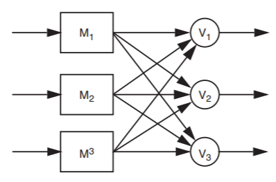
These calculations assume that the voter is perfectly reliable. Rather than trying to create perfect voters, the obvious thing to do is replicate them, too. In fact, everything—modules, inputs, outputs, sensors, actuators, etc.—should be replicated, and the final vote should be taken by the client of the system. Thus, three-engine airplanes vote with their propellers: when one engine fails, the two that continue to operate overpower the inoperative one. On the input side, the pilot’s hand presses forward on three separate throttle levers. A fully replicated TMR supermodule is shown in Figure \(\PageIndex{5}\). With this interconnection arrangement, any measurement or estimate of the reliability, \(R\), of a component module should include the corresponding voter. It is actually customary (and more logical) to consider a voter to be a component of the next module in the chain rather than, as the diagram suggests, the previous module. This fully replicated design is sometimes described as recursive.

Figure \(\PageIndex{5}\): Triple-modular redundant supermodule, with three inputs, three voters, and three outputs.

The numerical effect of fail-vote TMR is impressive. If the reliability of a single module at time T is 0.999, Equation \(\PageIndex{1}\) says that the reliability of a fail-vote TMR supermodule at that same time is 0.999997. TMR has reduced the probability of failure from one in a thousand to three in a million. This analysis explains why airplanes intended to fly across the ocean have more than one engine. Suppose that the rate of engine failures is such that a single-engine plane would fail to complete one out of a thousand trans-Atlantic flights. Suppose also that a 3-engine plane can continue flying as long as any 2 engines are operating, but it is too heavy to fly with only 1 engine. In 3 flights out of a thousand, one of the three engines will fail, but if engine failures are independent, in 999 out of each thousand first-engine failures, the remaining 2 engines allow the plane to limp home successfully.

Although TMR has greatly improved reliability, it has not made a comparable impact on MTTF. In fact, the MTTF of a fail-vote TMR supermodule can be smaller than the MTTF of the original, single-replica module. The exact effect depends on the failure process of the replicas, so for illustration consider a memoryless failure process, not because it is realistic but because it is mathematically tractable. Suppose that airplane engines have an MTTF of 6,000 hours, they fail independently, the mechanism of engine failure is memoryless, and (since this is a fail-vote design) we need at least 2 operating engines to get home. When flying with three engines, the plane accumulates 6,000 hours of engine running time in only 2,000 hours of flying time, so from the point of view of the airplane as a whole, 2,000 hours is the expected time to the first engine failure. While flying with the remaining two engines, it will take another 3,000 flying hours to accumulate 6,000 more engine hours. Because the failure process is memoryless we can calculate the MTTF of the 3-engine plane by adding:

Mean time to first failure	2000 hours (three engines)
Mean time from first to second failure	3000 hours (two engines)
Total mean time to system failure	5000 hours

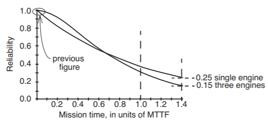
Thus the mean time to system failure is less than the 6,000 hour MTTF of a single engine. What is going on here is that we have actually sacrificed long-term reliability in order to enhance short-term reliability. Figure \(\PageIndex{6}\) illustrates the reliability of our hypothetical airplane during its 6 hours of flight, which amounts to only 0.001 of the single-engine MTTF—the mission time is very short compared with the MTTF and the reliability is far higher. Figure \(\PageIndex{7}\) shows the same curve, but for flight times that are comparable with the MTTF. In this region, if the plane tried to keep flying for 8000 hours (about 1.4 times the single-engine MTTF), a single-engine plane would fail to complete the flight in 3 out of 4 tries, but the 3-engine plane would fail to complete the flight in 5 out of 6 tries. (One should be wary of these calculations because the assumptions of independence and memoryless operation may not be met in practice. Sidebar \(\PageIndex{1}\) elaborates.)

Figure \(\PageIndex{6}\): Reliability with triple modular redundancy, for mission times much less than the MTTF of 6,000 hours. The vertical dotted line represents a six-hour flight.

Figure \(\PageIndex{7}\): Reliability with triple modular redundancy, for mission times comparable to the MTTF of 6,000 hours. The two vertical dotted lines represent mission times of 6,000 hours (left) and 8,400 hours (right).

Sidebar \(\PageIndex{1}\)

Risks of manipulating MTTFs

The apparently casual manipulation of MTTFs in Sections 2.5.3 and 2.5.4 is justified by assumptions of independence of failures and memoryless processes. But one can trip up by blindly applying this approach without understanding its limitations. To see how, consider a computer system that has been observed for several years to have a hardware crash an average of every 2 weeks and a software crash an average of every 6 weeks. The operator does not repair the system, but simply restarts it and hopes for the best. The composite MTTF is 1.5 weeks, determined most easily by considering what happens if we run the system for, say, 60 weeks. During that time we expect to see

• 10 software failures
• 30 hardware failures

_____________________

• 40 system failures in 60 weeks \(\rightarrow\) 1.5 weeks between failures

New hardware is installed, identical to the old except that it never fails. The MTTF should jump to 6 weeks because the only remaining failures are software, right?

Perhaps—but only if the software failure process is independent of the hardware failure process.

Suppose the software failure occurs because there is a bug (fault) in a clock-updating procedure: The bug always crashes the system exactly 420 hours (2.5 weeks) after it is started—if it gets a chance to run that long. The old hardware was causing crashes so often that the software bug only occasionally had a chance to do its thing—only about once every 6 weeks. Most of the time, the recovery from a hardware failure, which requires restarting the system, had the side effect of resetting the process that triggered the software bug. So, when the new hardware is installed, the system has an MTTF of only 2.5 weeks, much less than hoped.

MTTFs are useful, but one must be careful to understand what assumptions go into their measurement and use.

If we had assumed that the plane could limp home with just one engine, the MTTF would have increased, rather than decreased, but only modestly. Replication provides a dramatic improvement in reliability for missions of duration short compared with the MTTF, but the MTTF itself changes much less. We can verify this claim with a little more analysis, again assuming memoryless failure processes to make the mathematics tractable. Suppose we have an NMR system with the property that it somehow continues to be useful as long as at least one replica is still working. (This system requires using failfast replicas and a cleverer voter, as described in Section 2.5.4 below.) If a single replica has an \(MTTF_{replica} = 1\), there are \(N\) independent replicas, and the failure process is memoryless, the expected time until the first failure is \(MTTF_{replica}/N\), the expected time from then until the second failure is \(MTTF_{replica}/(N - 1)\), etc., and the expected time until the system of \(N\) replicas fails is the sum of these times,

\[ MTTF_{system} = 1 + 1/2 + 1/3 + \dots (1-N) \]

which for large \(N\) is approximately \(\ln (N)\). As we add to the cost by adding more replicas, \(MTTF_{system}\) grows disappointingly slowly—proportional to the logarithm of the cost. To multiply the \(MTTF_{system}\) by \(K\), the number of replicas required is \(e^K\) —the cost grows exponentially. The significant conclusion is that in systems for which the mission time is long compared with \(MTTF_{replica},\) simple replication escalates the cost while providing little benefit. On the other hand, there is a way of making replication effective for long missions, too. The method is to enhance replication by adding repair.

 

Repair

Let us return now to a fail-vote TMR supermodule (that is, it requires that at least two replicas be working) in which the voter has just noticed that one of the three replicas is producing results that disagree with the other two. Since the voter is in a position to report which replica has failed, suppose that it passes such a report along to a repair person who immediately examines the failing replica and either fixes or replaces it. For this approach, the mean time to repair (MTTR) measure becomes of interest. The supermodule fails if either the second or third replica fails before the repair to the first one can be completed. Our intuition is that if the MTTR is small compared with the combined MTTF of the other two replicas, the chance that the supermodule fails will be similarly small.

The exact effect on chances of supermodule failure depends on the shape of the reliability function of the replicas. In the case where the failure and repair processes are both memoryless, the effect is easy to calculate. Since the rate of failure of 1 replica is \(1/MTTF\), the rate of failure of 2 replicas is \(2/MTTF\). If the repair time is short compared with MTTF, the probability of a failure of one of the two remaining replicas while waiting a time \(T\) for repair of the one that failed is approximately \(2T/MTTF\). Since the mean time to repair is MTTR, we have

\[ Pr( \text{supermodule fails while waiting for repair} ) = \frac{2 \times MTTR}{MTTF} \]

Continuing our airplane example and temporarily suspending disbelief, suppose that during a long flight we send a mechanic out on the airplane’s wing to replace a failed engine. If the replacement takes 1 hour, the chance that one of the other two engines fails during that hour is approximately 1/3000. Moreover, once the replacement is complete, we expect to fly another 2000 hours until the next engine failure. Assuming further that the mechanic is carrying an unlimited supply of replacement engines, completing a 10,000 hour flight—or even a longer one—becomes plausible. The general formula for the MTTF of a fail-vote TMR supermodule with memoryless failure and repair processes is (this formula comes out of the analysis of continuous-transition birth-and-death Markov processes, an advanced probability technique that is beyond our scope):

\[ MTTF_{\text{supermodule}} = \frac{MTTF_{replica}}{3} \times \frac{MTTF_{replica}}{2 \times MTTR_{replica}} = \frac{(MTTF_{replica})^2}{6 \times MTTR_{replica}} \]

Thus, our 3-engine plane with hypothetical in-flight repair has an MTTF of 6 million hours, an enormous improvement over the 6000 hours of a single-engine plane. This equation can be interpreted as saying that, compared with an unreplicated module, the MTTF has been reduced by the usual factor of 3 because there are 3 replicas, but at the same time the availability of repair has increased the MTTF by a factor equal to the ratio of the MTTF of the remaining 2 engines to the MTTR.

Replacing an airplane engine in flight may be a fanciful idea, but replacing a magnetic disk in a computer system on the ground is quite reasonable. Suppose that we store 3 replicas of a set of data on 3 independent hard disks, each of which has an MTTF of 5 years (using as the MTTF the expected operational lifetime, not the "MTTF" derived from the short-term failure rate). Suppose also, that if a disk fails, we can locate, install, and copy the data to a replacement disk in an average of 10 hours. In that case, by Equation \(\PageIndex{5}\), the MTTF of the data is

\[ \frac{(MTTF_{replica})^2}{6 \times MTTR_{replica}} = \frac{(5 \ \text{years})^2}{6 \cdot (10 \ \text{hours}) / (8760 \ \text{hours/year})} = 3650 \ \text{years} \]

In effect, redundancy plus repair has reduced the probability of failure of this supermodule to such a small value that for all practical purposes, failure can be neglected and the supermodule can operate indefinitely.

Before running out to start a company that sells superbly reliable disk-storage systems, it would be wise to review some of the overly optimistic assumptions we made in getting that estimate of the MTTF, most of which are not likely to be true in the real world:

• Disks fail independently. A batch of real world disks may all come from the same vendor, where they acquired the same set of design and manufacturing faults. Or, they may all be in the same machine room, where a single earthquake—which probably has an MTTF of less than 3,650 years—may damage all three.
• Disk failures are memoryless. Real-world disks follow a bathtub curve. If, when disk #1 fails, disk #2 has already been in service for three years, disk #2 no longer has an expected operational lifetime of 5 years, so the chance of a second failure while waiting for repair is higher than the formula assumes. Furthermore, when disk #1 is replaced, its chances of failing are probably higher than usual for the first few weeks.
• Repair is also a memoryless process. In the real world, if we stock enough spares that we run out only once every 10 years and have to wait for a shipment from the factory, but doing a replacement happens to run us out of stock today, we will probably still be out of stock tomorrow and the next day.
• Repair is done flawlessly. A repair person may replace the wrong disk, forget to copy the data to the new disk, or install a disk that hasn’t passed burn-in and fails in the first hour.

Each of these concerns acts to reduce the reliability below what might be expected from our overly simple analysis. Nevertheless, NMR with repair remains a useful technique, and in Chapter 4 we will see ways in which it can be applied to disk storage. 

One of the most powerful applications of NMR is in the masking of transient errors. When a transient error occurs in one replica, the NMR voter immediately masks it. Because the error is transient, the subsequent behavior of the supermodule is as if repair happened by the next operation cycle. The numerical result is little short of extraordinary. For example, consider a processor arithmetic logic unit (ALU) with a 1 gigahertz clock and which is triply replicated with voters checking its output at the end of each clock cycle. In Equation \(\PageIndex{5}\) we have \(MTTR_{replica} = 1\) (in this application, Equation \(\PageIndex{5}\) is only an approximation because the time to repair is a constant rather than the result of a memoryless process), and \(MTTF_{supermodule} = (MTTF_{replica})^2 ⁄ 6 \ \text{cycles}\). If \(MTTF_{replica}\) is 10¹⁰ cycles (1 error in 10 billion cycles, which at this clock speed means one error every 10 seconds), \(MTTF_{supermodule}\) is 10²⁰ ⁄ 6 cycles, about 500 years. TMR has taken three ALUs that were for practical use nearly worthless and created a super-ALU that is almost infallible.

The reason things seem so good is that we are evaluating the chance that two transient errors occur in the same operation cycle. If transient errors really are independent, that chance is small. This effect is powerful, but the leverage works in both directions, thereby creating a potential hazard: it is especially important to keep track of the rate at which transient errors actually occur. If they are happening, say, 20 times as often as hoped, \(MTTF_{supermodule}\) will be 1/400 of the original prediction—the super-ALU is likely to fail once per year. That may still be acceptable for some applications, but it is a big change. Also, as usual, the assumption of independence is absolutely critical. If all the ALUs came from the same production line, it seems likely that they will have at least some faults in common, in which case the super-ALU may be just as worthless as the individual ALUs.

Several variations on the simple fail-vote structure appear in practice:

• Purging. In an NMR design with a voter, whenever the voter detects that one replica disagrees with the majority, the voter calls for its repair and in addition marks that replica DOWN and ignores its output until hearing that it has been repaired. This technique doesn’t add anything to a TMR design, but with higher levels of replication, as long as replicas fail one at a time and any two replicas continue to operate correctly, the supermodule works.
• Pair-and-compare. Create a fail-fast module by taking two replicas, giving them the same inputs, and connecting a simple comparator to their outputs. As long as the comparator reports that the two replicas of a pair agree, the next stage of the system accepts the output. If the comparator detects a disagreement, it reports that the module has failed. The major attraction of pair-and-compare is that it can be used to create fail-fast modules starting with easily available commercial, off-the-shelf components, rather than commissioning specialized fail-fast versions. Special high-reliability components typically have a cost that is much higher than off-the-shelf designs, for two reasons. First, since they take more time to design and test, the ones that are available are typically of an older, more expensive technology. Second, they are usually low-volume products that cannot take advantage of economies of large-scale production. These considerations also conspire to produce long delivery cycles, making it harder to keep spares in stock. An important aspect of using standard, high-volume, low-cost components is that one can afford to keep a stock of spares, which in turn means that MTTR can be made small: just replace a failing replica with a spare (the popular term for this approach is pair-and-spare) and do the actual diagnosis and repair at leisure.
• NMR with fail-fast replicas. If each of the replicas is itself a fail-fast design (perhaps using pair-and-compare internally), then a voter can restrict its attention to the outputs of only those replicas that claim to be producing good results and ignore those that are reporting that their outputs are questionable. With this organization, a TMR system can continue to operate even if 2 of its 3 replicas have failed, since the 1 remaining replica is presumably checking its own results. An NMR system with repair and constructed of fail-fast replicas is so robust that it is unusual to find examples for which \(N\) is greater than 2.

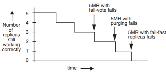
Figure \(\PageIndex{8}\) compares the ability to continue operating until repair arrives of 5MR designs that use fail-vote, purging, and fail-fast replicas. The observant reader will note that this chart can be deemed guilty of a misleading comparison, since it claims that the 5MR system continues working when only one fail-fast replica is still running. But if that fail-fast replica is actually a pair-and-compare module, it might be more accurate to say that there are two still-working replicas at that point. 

Figure \(\PageIndex{8}\): Failure points of three different 5MR supermodule designs, if repair does not happen in time.

Another technique that takes advantage of repair, can improve availability, and can degrade gracefully (in other words, it can be fail-soft) is called partition. If there is a choice of purchasing a system that has either one fast processor or two slower processors, the two-processor system has the virtue that when one of its processors fails, the system can continue to operate with half of its usual capacity until someone can repair the failed processor. An electric power company, rather than installing a single generator of capacity \(K\) megawatts, may install \(N\) generators of capacity \(K/N\) megawatts each.

When equivalent modules can easily share a load, partition can extend to what is called \(\bf{N + 1}\) redundancy. Suppose a system has a load that would require the capacity of \(N\) equivalent modules. The designer partitions the load across \(N + 1\) or more modules. Then, if any one of the modules fails, the system can carry on at full capacity until the failed module can be repaired.

\(N + 1\) redundancy is most applicable to modules that are completely interchangeable, can be dynamically allocated, and are not used as storage devices. Examples are processors, dial-up modems, airplanes, and electric generators. Thus, one extra airplane located at a busy hub can mask the failure of any single plane in an airline’s fleet. When modules are not completely equivalent (for example, electric generators come in a range of capacities, but can still be interconnected to share load), the design must ensure that the spare capacity is greater than the capacity of the largest individual module. For devices that provide storage, such as a hard disk, it is also possible to apply partition and \(N + 1\) redundancy with the same goals, but it requires a greater level of organization to preserve the stored contents when a failure occurs, for example by using RAID, as was described in Section 2.5.1, or some more general replica management system such as those discussed in Section 4.4.7.

For some applications an occasional interruption of availability is acceptable, while in others every interruption causes a major problem. When repair is part of the fault tolerance plan, it is sometimes possible, with extra care and added complexity, to design a system to provide continuous operation. Adding this feature requires that when failures occur, one can quickly identify the failing component, remove it from the system, repair it, and reinstall it (or a replacement part) all without halting operation of the system. The design required for continuous operation of computer hardware involves connecting and disconnecting cables and turning off power to some components but not others, without damaging anything. When hardware is designed to allow connection and disconnection from a system that continues to operate, it is said to allow hot swap.

In a computer system, continuous operation also has significant implications for the software. Configuration management software must anticipate hot swap so that it can stop using hardware components that are about to be disconnected, as well as discover newly attached components and put them to work. In addition, maintaining state is a challenge. If there are periodic consistency checks on data, those checks (and repairs to data when the checks reveal inconsistencies) must be designed to work correctly even though the system is in operation and the data is perhaps being read and updated by other users at the same time.

Overall, continuous operation is not a feature that should be casually added to a list of system requirements. When someone suggests it, it may be helpful to point out that it is much like trying to keep an airplane flying indefinitely. Many large systems that appear to provide continuous operation are actually designed to stop occasionally for maintenance.