
2.2: Linear Pulse Propagation in Isotropic Media
- Page ID
- 44643

For dielectric non-magnetic media, with no free charges and currents due to free charges, there is \(\vec{M} = \vec{0}, \vec{j} = \vec{0}, \rho = 0\). We obtain with \(\vec{D} = \epsilon (\vec{r}) \vec{E} = \epsilon_0 \epsilon_r (\vec{r}) \vec{E}\).
\[\vec{\nabla} \cdot (\epsilon (\vec{r}) \vec{E}) = 0. \nonumber \]
In addition for homogeneous media, we obtain \(\vec{\nabla} \cdot \vec{E} = 0\) and the wave equation (2.1.8) greatly simplifies
\[\left ( \Delta - \dfrac{1}{c_0^2} \dfrac{\partial^2}{\partial t^2} \right ) \vec{E} = \mu_0 \dfrac{\partial^2}{\partial t^2} \vec{P}. \label{eq2.2.2} \]
This is the wave equation driven by the polarization in the medium. If the medium is linear and has only an induced polarization described by the susceptibility \(\chi (\omega) = \epsilon_r (\omega) - 1\), we obtain in the frequency domain
\[\hat{\vec{P}} (\omega) = \epsilon_0 \chi (\omega) \hat{\vec{E}} (\omega). \nonumber \]
Substituted in Equation \ref{eq2.2.2}
\[\left (\Delta + \dfrac{\omega^2}{c_0^2} \right )\hat{\vec{E}} (\omega) = -\omega^2 \mu_0 \epsilon_0 \chi (\omega) \hat{\vec{E}}, \nonumber \]
where \(\hat{\vec{D}} = \epsilon_0 \epsilon_r (\omega) \hat{\vec{E}}\), and thus
\[\left (\Delta + \dfrac{\omega^2}{c_0^2} (1 + \chi (\omega)\right ) \widehat{\vec{E}} = 0, \nonumber \]
with the refractive index \(n\) and \(1 + \chi (\omega) = n^2\)
\[\left (\Delta + \dfrac{\omega^2}{c^2} \right ) \hat{\vec{E}} = 0 \nonumber \]
where \(c = c_0/n\) is the velocity of light in the medium.
Plane-Wave Solutions (TEM-Waves)
The complex plane-wave solution of Equation (2.2.6) is given by
\[\hat{\vec{E}}^{(+)} (\omega, \vec{r}) = \hat{\vec{E}}^{(+)} (\omega) e^{-j \vec{k} \cdot \vec{r}} = E_0 e^{-j \vec{k} \cdot \vec{r}} \cdot \vec{e} \nonumber \]
with
\[|\vec{k}|^2 = \dfrac{\omega^2}{c^2} = k^2. \nonumber \]
Thus, the dispersion relation is given by
\[k(\omega) = \dfrac{\omega}{c_0} n (\omega). \nonumber \]
From \(\vec{\nabla} \cdot \vec{E} = 0\), we see that \(\vec{k} \perp \vec{e}\). In time domain, we obtain
\[\vec{E}^{(+)} (\vec{r}, t) = E_0 \vec{e} \cdot e^{j\omega t - j \vec{k} \cdot \vec{r}} \nonumber \]
with
\[k = 2\pi /\lambda, \nonumber \]
where \(\lambda\) is the wavelength, \(\omega\) the angular frequency, \(\vec{k}\) the wave vector, \(\vec{e}\) the polarization vector, and \(f = \omega /2\pi\) the frequency. From Equation (2.1.2), we get for the magnetic field
\[-j \vec{k} \times E_0 \vec{e} e^{j(\omega t - \vec{k} \vec{r})} = -j \mu_0 \omega \vec{H}^{(+)}, \nonumber \]
or
\[\vec{H}^{(+)} = \dfrac{E_0}{\mu_0 \omega} e^{j(\omega t - \vec{k}\vec{r})} \vec{k} \times \vec{e} = H_0 \vec{h} e^{j(\omega t - \vec{k}\vec{r})} \nonumber \]
with
\[\vec{h} = \dfrac{\vec{k}}{|k|} \times \vec{e} \nonumber \]
and
\[H_0 = \dfrac{|k|}{\mu_0 \omega} E_0 = \dfrac{1}{Z_F E_0}. \nonumber \]
The natural impedance is
\[Z_F = \mu_0 c = \sqrt{\dfrac{\mu_0}{\epsilon_0 \epsilon_r}} = \dfrac{1}{n} Z_{F_0} \nonumber \]
with the free space impedance
\[Z_{F_0} = \sqrt{\dfrac{\mu_0}{\epsilon_0}} = 377 \Omega. \nonumber \]
For a backward propagating wave with \(\vec{E}^{(+)} (\vec{r}, t) = E_0 \vec{e} \cdot e^{j \omega t + j \vec{k} \cdot \vec{r}}\) there is \(\vec{H}^{(+)} = H_0 \vec{h} e^{j (\omega t - \vec{k} \vec{r})}\) with
\[H_0 = -\dfrac{|k|}{\mu_0 \omega} E_0. \nonumber \]
Note that the vectors \(\vec{e}, \vec{h}\) and \(\vec{k}\) form an orthogonal trihedral,
\[\vec{e} \perp \vec{h}, \vec{k} \perp \vec{e}, \vec{k} \perp \vec{h}. \nonumber \]
Complex Notations
Physical \(\vec{E}, \vec{H}\) fields are real:
\[\vec{E} (\vec{r}, t) = \dfrac{1}{2}\left (\vec{E}^{(+)} (\vec{r}, t) + \vec{E}^{(-)} (\vec{r}, t)\right ) \nonumber \]
with \(\vec{E}^{(-)} (\vec{r}, t) = \vec{E}^{(+)} (\vec{r}, t)^*\). A general temporal shape can be obtained by adding different spectral components,
\[\vec{E}^{(+)} (\vec{r}, t) = \int_{0}^{\infty} \dfrac{d\omega}{2\pi} \hat{\vec{E}}^{(+)} (\omega) e^{j(\omega t - \vec{k} \cdot \vec{r})} \nonumber \]
Correspondingly, the magnetic field is given by
\[\vec{H} (\vec{r}, t) = \dfrac{1}{2} \left (\vec{H}^{(+)} (\vec{r}, t) + \vec{H}^{(-)} (\vec{r}, t) \right ) \nonumber \]
with \(\vec{H}^{(-)} (\vec{r}, t) = \vec{H}^{(+)} (\vec{r}, t)^*\). The general solution is given by
\[\vec{H}^{(+)} (\vec{r}, t) = \int_{0}^{\infty} \dfrac{d\omega}{2\pi} \hat{\vec{H}}^{(+)} (\omega) e^{j(\omega t - \vec{k} \cdot \vec{r})} \nonumber \]
with
\[\hat{\vec{H}}^{(+)} (\omega) = \dfrac{E_0}{Z_F} \vec{h}. \nonumber \]
Poynting Vectors, Energy Density and Intensity for Plane Wave Fields
| Quantity | Real fields | Complex fields \(\langle \rangle_t\) |
|---|---|---|
| Energy density | \(w = \dfrac{1}{2} (\epsilon_0 \epsilon_r \vec{E}^2 + \mu_0 \mu_r \vec{H}^2)\) | \(w = \dfrac{1}{4} (\epsilon_0 \epsilon_r |\vec{E}^{(+)}|^2 + \mu_0 \mu_r |\vec{H}^{(+)}|^2)\) |
| Poynting vector | \(\vec{S} = \vec{E} \times \vec{H}\) | \(\vec{T} = \dfrac{1}{2} \vec{E}^{(+)} \times (\vec{H}^{(+)})^*\) |
| Intensity | \(I = |\vec{S}| = cw\) | \(I = |vec{T}| = cw\) |
| Energy Cons | \(\dfrac{\partial w}{\partial t} + \vec{\nabla} \vec{S} = 0\) | \(\dfrac{\partial w}{\partial t} + \vec{\nabla} \vec{T} = 0\) |
For \(\vec{E}^{(+)} (\vec{r}, t) = E_0 \vec{e}_x e^{j (\omega t - kz)}\) we obtain the energy density
\[w = \dfrac{1}{2} \epsilon_r \epsilon_0 |E_0|^2, \nonumber \]
the poynting vector
\[\vec{T} = \dfrac{1}{2Z_F} |E_0|^2 \vec{e}_z \nonumber \]
and the intensity
\[I = \dfrac{1}{2Z_F} |E_0|^2 = \dfrac{1}{2} Z_F |H_0|^2. \nonumber \]
Dielectric Susceptibility
The polarization is given by
\[\vec{P}^{(+)} (\omega) = \dfrac{\text{dipole moment}}{\text{volume}} = N \cdot \langle \vec{p}^{(+)} (\omega)\rangle = \epsilon_0 \chi (\omega) \vec{E}^{(+)} (\omega), \nonumber \]
where \(N\) is density of elementary units and \(\langle \vec{p} \rangle\) is the average dipole moment of unit (atom, molecule, ...).
Classical harmonic oscillator model
The damped harmonic oscillator driven by an electric force in one dimension, \(x\), is described by the differential equation
\[m \dfrac{d^2 x}{dt^2} + 2 \dfrac{\omega_0}{Q} m \dfrac{dx}{dt} + m \omega_0^2 x = e_0 E(t), \nonumber \]
where \(E(t) = \hat{E} e^{j \omega t}\). By using the ansatz \(x(t) = \hat{x} e^{j\omega t}\), we obtain for the complex amplitude of the dipole moment \(p = e_0 x(t) = \hat{p} e^{j\omega t}\)
\[\hat{p} = \dfrac{\tfrac{e_0^2}{m}}{(\omega_0^2 - \omega^2) + 2j \tfrac{\omega_0}{Q} \omega} \hat{E}. \nonumber \]
For the susceptibility, we get
\[\chi (\omega) = \dfrac{N \tfrac{e_0^2}{m} \tfrac{1}{\epsilon_0}}{(\omega_0^2 - \omega^2) + 2j \omega \tfrac{\omega_0}{Q}} \nonumber \]
and thus
\[\chi (\omega) = \dfrac{\omega_p^2}{(\omega_0^2 - \omega^2) + 2j \omega \tfrac{\omega_0}{Q}}\label{eq2.2.32} \]
with the plasma frequency \(\omega_p\), determined by \(\omega_p^2 = N e_0^2 /m \epsilon_0\). Figure 2.1 shows the real part and imaginary part of the classical susceptiblity (Equation \(\ref{eq2.2.32}\)).
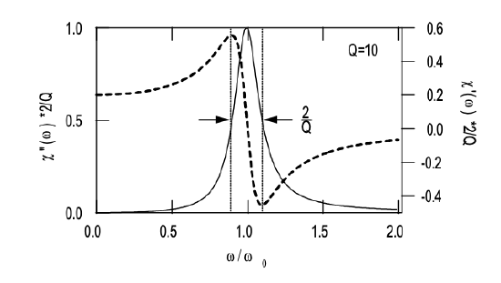
Note, there is a small resonance shift due to the loss. Off resonance, the imaginary part approaches very quickly zero. Not so the real part, it approaches a constant value \(\omega_p^2/\omega_0^2\) below resonance, and approaches zero for above resonance, but slower than the real part, i.e. off resonance there is still a contribution to the index but practically no loss.