
2.3: Bloch Equations
- Page ID
- 44644
\( \newcommand{\vecs}[1]{\overset { \scriptstyle \rightharpoonup} {\mathbf{#1}} } \)
\( \newcommand{\vecd}[1]{\overset{-\!-\!\rightharpoonup}{\vphantom{a}\smash {#1}}} \)
\( \newcommand{\dsum}{\displaystyle\sum\limits} \)
\( \newcommand{\dint}{\displaystyle\int\limits} \)
\( \newcommand{\dlim}{\displaystyle\lim\limits} \)
\( \newcommand{\id}{\mathrm{id}}\) \( \newcommand{\Span}{\mathrm{span}}\)
( \newcommand{\kernel}{\mathrm{null}\,}\) \( \newcommand{\range}{\mathrm{range}\,}\)
\( \newcommand{\RealPart}{\mathrm{Re}}\) \( \newcommand{\ImaginaryPart}{\mathrm{Im}}\)
\( \newcommand{\Argument}{\mathrm{Arg}}\) \( \newcommand{\norm}[1]{\| #1 \|}\)
\( \newcommand{\inner}[2]{\langle #1, #2 \rangle}\)
\( \newcommand{\Span}{\mathrm{span}}\)
\( \newcommand{\id}{\mathrm{id}}\)
\( \newcommand{\Span}{\mathrm{span}}\)
\( \newcommand{\kernel}{\mathrm{null}\,}\)
\( \newcommand{\range}{\mathrm{range}\,}\)
\( \newcommand{\RealPart}{\mathrm{Re}}\)
\( \newcommand{\ImaginaryPart}{\mathrm{Im}}\)
\( \newcommand{\Argument}{\mathrm{Arg}}\)
\( \newcommand{\norm}[1]{\| #1 \|}\)
\( \newcommand{\inner}[2]{\langle #1, #2 \rangle}\)
\( \newcommand{\Span}{\mathrm{span}}\) \( \newcommand{\AA}{\unicode[.8,0]{x212B}}\)
\( \newcommand{\vectorA}[1]{\vec{#1}} % arrow\)
\( \newcommand{\vectorAt}[1]{\vec{\text{#1}}} % arrow\)
\( \newcommand{\vectorB}[1]{\overset { \scriptstyle \rightharpoonup} {\mathbf{#1}} } \)
\( \newcommand{\vectorC}[1]{\textbf{#1}} \)
\( \newcommand{\vectorD}[1]{\overrightarrow{#1}} \)
\( \newcommand{\vectorDt}[1]{\overrightarrow{\text{#1}}} \)
\( \newcommand{\vectE}[1]{\overset{-\!-\!\rightharpoonup}{\vphantom{a}\smash{\mathbf {#1}}}} \)
\( \newcommand{\vecs}[1]{\overset { \scriptstyle \rightharpoonup} {\mathbf{#1}} } \)
\(\newcommand{\longvect}{\overrightarrow}\)
\( \newcommand{\vecd}[1]{\overset{-\!-\!\rightharpoonup}{\vphantom{a}\smash {#1}}} \)
\(\newcommand{\avec}{\mathbf a}\) \(\newcommand{\bvec}{\mathbf b}\) \(\newcommand{\cvec}{\mathbf c}\) \(\newcommand{\dvec}{\mathbf d}\) \(\newcommand{\dtil}{\widetilde{\mathbf d}}\) \(\newcommand{\evec}{\mathbf e}\) \(\newcommand{\fvec}{\mathbf f}\) \(\newcommand{\nvec}{\mathbf n}\) \(\newcommand{\pvec}{\mathbf p}\) \(\newcommand{\qvec}{\mathbf q}\) \(\newcommand{\svec}{\mathbf s}\) \(\newcommand{\tvec}{\mathbf t}\) \(\newcommand{\uvec}{\mathbf u}\) \(\newcommand{\vvec}{\mathbf v}\) \(\newcommand{\wvec}{\mathbf w}\) \(\newcommand{\xvec}{\mathbf x}\) \(\newcommand{\yvec}{\mathbf y}\) \(\newcommand{\zvec}{\mathbf z}\) \(\newcommand{\rvec}{\mathbf r}\) \(\newcommand{\mvec}{\mathbf m}\) \(\newcommand{\zerovec}{\mathbf 0}\) \(\newcommand{\onevec}{\mathbf 1}\) \(\newcommand{\real}{\mathbb R}\) \(\newcommand{\twovec}[2]{\left[\begin{array}{r}#1 \\ #2 \end{array}\right]}\) \(\newcommand{\ctwovec}[2]{\left[\begin{array}{c}#1 \\ #2 \end{array}\right]}\) \(\newcommand{\threevec}[3]{\left[\begin{array}{r}#1 \\ #2 \\ #3 \end{array}\right]}\) \(\newcommand{\cthreevec}[3]{\left[\begin{array}{c}#1 \\ #2 \\ #3 \end{array}\right]}\) \(\newcommand{\fourvec}[4]{\left[\begin{array}{r}#1 \\ #2 \\ #3 \\ #4 \end{array}\right]}\) \(\newcommand{\cfourvec}[4]{\left[\begin{array}{c}#1 \\ #2 \\ #3 \\ #4 \end{array}\right]}\) \(\newcommand{\fivevec}[5]{\left[\begin{array}{r}#1 \\ #2 \\ #3 \\ #4 \\ #5 \\ \end{array}\right]}\) \(\newcommand{\cfivevec}[5]{\left[\begin{array}{c}#1 \\ #2 \\ #3 \\ #4 \\ #5 \\ \end{array}\right]}\) \(\newcommand{\mattwo}[4]{\left[\begin{array}{rr}#1 \amp #2 \\ #3 \amp #4 \\ \end{array}\right]}\) \(\newcommand{\laspan}[1]{\text{Span}\{#1\}}\) \(\newcommand{\bcal}{\cal B}\) \(\newcommand{\ccal}{\cal C}\) \(\newcommand{\scal}{\cal S}\) \(\newcommand{\wcal}{\cal W}\) \(\newcommand{\ecal}{\cal E}\) \(\newcommand{\coords}[2]{\left\{#1\right\}_{#2}}\) \(\newcommand{\gray}[1]{\color{gray}{#1}}\) \(\newcommand{\lgray}[1]{\color{lightgray}{#1}}\) \(\newcommand{\rank}{\operatorname{rank}}\) \(\newcommand{\row}{\text{Row}}\) \(\newcommand{\col}{\text{Col}}\) \(\renewcommand{\row}{\text{Row}}\) \(\newcommand{\nul}{\text{Nul}}\) \(\newcommand{\var}{\text{Var}}\) \(\newcommand{\corr}{\text{corr}}\) \(\newcommand{\len}[1]{\left|#1\right|}\) \(\newcommand{\bbar}{\overline{\bvec}}\) \(\newcommand{\bhat}{\widehat{\bvec}}\) \(\newcommand{\bperp}{\bvec^\perp}\) \(\newcommand{\xhat}{\widehat{\xvec}}\) \(\newcommand{\vhat}{\widehat{\vvec}}\) \(\newcommand{\uhat}{\widehat{\uvec}}\) \(\newcommand{\what}{\widehat{\wvec}}\) \(\newcommand{\Sighat}{\widehat{\Sigma}}\) \(\newcommand{\lt}{<}\) \(\newcommand{\gt}{>}\) \(\newcommand{\amp}{&}\) \(\definecolor{fillinmathshade}{gray}{0.9}\)Atoms in low concentration show line spectra as found in gas-, dye- and some solid-state laser media. Usually, there are infinitely many energy eigenstates in an atomic, molecular or solid-state medium and the spectral lines are associated with allowed transitions between two of these energy eigenstates. For many physical considerations it is already sufficient to take only two of the possible energy eigenstates into account, for example those which are related to the laser transition. The pumping of the laser can be described by phenomenological relaxation processes into the upper laser level and out of the lower laser level. The resulting simple model is often called a two-level atom, which is mathematically also equivalent to a spin 1/2 particle in an external magnetic field, because the spin can only be parallel or anti- parallel to the field, i.e. it has two energy levels and energy eigenstates. The interaction of the two-level atom or the spin with the electric or magnetic field is described by the Bloch equations.
Two-Level Model
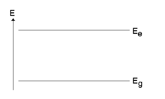
An atom having only two energy eigenvalues is described by a two-dimensional state space spanned by the two energy eigenstates |\(e\) \rangle and |\(g\) \rangle . The two states constitute a complete orthonormal system. The corresponding energy eigenvalues are \(E_e\) and \(E_g\) (Figure 2.2).
In the position-, i.e. x-representation, these states correspond to the wave functions
\[\psi_e(x) = \langle x|e \rangle , \ \ \ \ \ \text{ and } \psi_g(x) = \langle x|g \rangle .\label{eq2.3.1} \]
The Hamiltonian of the atom is given by
\[H_A = E_e |e\rangle \langle e| + E_g |g\rangle \langle g|. \nonumber \]
In this two-dimensional state space only \(2 \times 2 = 4\) linearly independent linear operators are possible. A possible choice for an operator base in this space is
\[1 = |e \rangle \langle e| + |g\rangle \langle g|, \nonumber \]
\[\sigma_z = |e\rangle \langle e| - |g\rangle \langle g|,\label{eq2.3.4} \]
\[\sigma^+ = |e\rangle \langle g|, \nonumber \]
\[\sigma^- = |g\rangle \langle e|.\label{eq2.3.6} \]
The non-Hermitian operators \(\sigma^{\pm}\) could be replaced by the Hermitian operators \(\sigma_{x,y}\)
\[\sigma_x = \sigma^+ + \sigma^-, \nonumber \]
\[\sigma_y = -j\sigma^+ + j\sigma^-. \nonumber \]
The physical meaning of these operators becomes obvious, if we look at the action when applied to an arbitrary state
\[|\psi \rangle = c_g |g \rangle + c_e| e\rangle .\label{eq2.3.9} \]
We obtain
\[\sigma^+|\psi \rangle = c_g|e\rangle , \nonumber \]
\[\sigma^-|\psi \rangle = c_e|g\rangle , \nonumber \]
\[\sigma_z|\psi \rangle = c_e|e\rangle -c_g |g\rangle . \nonumber \]
The operator \(\sigma^+\) generates a transition from the ground to the excited state, and \(\sigma^-\) does the opposite. In contrast to \(\sigma^+\) and \(\sigma^-\), \(\sigma_z\) is a Hermitian operator, and its expectation value is an observable physical quantity with expectation value
\[\langle \psi |\sigma_z| \psi \rangle = |c_e|^2 - |c_g|^2 = \omega, \nonumber \]
the inversion \(\omega\) of the atom, since \(|c_e|^2\) and \(|c_g|^2\) are the probabilities for finding the atom in state \(|e \rangle \) or \(|g \rangle \) upon a corresponding measurement.
If we consider an ensemble of \(N\) atoms the total inversion would be \(\sigma = N\langle \psi |\sigma_z| \psi \rangle \). If we separate from the Hamiltonian (Equation \(\ref{eq2.3.1}\)) the term \((E_e + E_g)/2 \cdot 1\), where 1 denotes the the unity matrix, we rescale the energy values correspondingly and obtain for the Hamiltonian of the two-level system
\[H_A = \dfrac{1}{2} \hat{h} \omega_{eg} \sigma_z, \nonumber \]
with the transition frequency
\[\omega_{eg} = \dfrac{1}{\hat{h}} (E_e - E_g). \nonumber \]
This form of the Hamiltonian is favorable. There are the following commutator relations between operators (Equation \(\ref{eq2.3.4}\)) to (Equation \(\ref{eq2.3.6}\))
\[[\sigma^+, \sigma^-] = \sigma_z,\label{eq2.3.16} \]
\[[\sigma^+, \sigma_z] = -2\sigma^+, \nonumber \]
\[[\sigma^-, \sigma_z] = 2\sigma^-,\label{eq2.3.18} \]
and anti-commutator relations, respectively
\[[\sigma^+, \sigma^-]_+ = 1, \nonumber \]
\[[\sigma^+, \sigma_z]_+ = 0, \nonumber \]
\[[\sigma^-, \sigma_z]_+ = 0, \nonumber \]
\[[\sigma^-, \sigma^-]_+ = [\sigma^+, \sigma^+]_+ = 0, \nonumber \]
The operators \(\sigma_x\), \(\sigma_y\), \(\sigma_z\) fulfill the angular momentum commutator relations
\[[\sigma_x, \sigma_y] = 2j \sigma_z, \nonumber \]
\[[\sigma_y, \sigma_z] = 2j \sigma_x, \nonumber \]
\[[\sigma_z, \sigma_x] = 2j \sigma_y, \nonumber \]
The two-dimensional state space can be represented as vectors in \(\mathbb{C}^2\) according to the rule:
\[|\psi \rangle = c_e| e\rangle + c_g|g \rangle \to \ \ \left (\begin{matrix} c_e \\ c_g \end{matrix} \right ). \nonumber \]
The operators are then represented by matrices
\[\sigma^+ \to \left ( \begin{matrix} 0 & 1 \\ 0 & 0 \end{matrix} \right ),\label{eq2.3.27} \]
\[\sigma^- \to \left ( \begin{matrix} 0 & 0 \\ 1 & 0 \end{matrix} \right ), \nonumber \]
\[\sigma_z \to \left ( \begin{matrix} 1 & 0 \\ 0 & -1 \end{matrix} \right ), \nonumber \]
\[1 \to \left ( \begin{matrix} 1 & 0 \\ 0 & 1 \end{matrix} \right ).\label{eq.2.3.30} \]
Atom-Field Interaction In Dipole Approximation
The dipole moment of an atom \(\tilde{P}\) is essentially determined by the position operator \(\vec{x}\) via
\[\vec{P} = -e_0 \vec{x}.\label{eq2.3.31} \]
Then the expectation value for the dipole moment of an atom in state (Equation \(\ref{eq2.3.9}\)) is
\[\begin{array} {rcl} {\langle \psi |\vec{P}|\psi \rangle } & = & {-e_0 (|c_e|^2 \langle e|\bar{x}|e \rangle + c_e c_g^* \langle g|\bar{x}| e\rangle } \\ {} & + & {c_gc_e^* \langle e|\bar{x}| g\rangle +|c_g|^2 \langle g|\bar{x}|g \rangle ).}\end{array} \nonumber \]
For simplicity, we may assume that that the medium is an atomic gas. The atoms posses inversion symmetry, therefore, energy eigenstates must be symmetric or anti-symmetric, i.e. \(\langle e|\bar{x}|e\rangle =\langle g|\bar{x}|g\rangle =0\). We obtain
\[\langle \psi |\bar{P} \psi\rangle = -e_0 (c_ec_g^* \langle g|\bar{x}|e\rangle + c_g c_e^* \langle g|\bar{x}|e\rangle ^*). \nonumber \]
(Note, this means, there is no permanent dipole moment in an atom, which is in an energy eigenstate. Note, this might not be the case in a solid. The atoms constituting the solid are oriented in a lattice, which may break the symmetry. If so, there are permanent dipole moments and consequently the matrix elements \(\langle e|\bar{x}|e \rangle \) and \(\langle g|\bar{x}|g \rangle \) would not vanish. If so, there are also crystal fields, which then imply level shifts, via the linear Stark effect.) Thus an atom does only exhibit a dipole moment in the average, if the product \(c_ec_g^* \ne 0\), i.e. the state of the atom is in a superposition of states \(|e \rangle \) and \(|g \rangle \).
With the dipole matrix elements
\[\bar{M} = e_0 \langle g|\bar{x}|e\rangle \nonumber \]
the expectation value for the dipole moment can be written as
\[\langle \psi |\bar{P}| \psi \rangle = -(c_e c_g^* \vec{M} + c_g c_e^* \vec{M}^*) = - \langle \psi |(\sigma^+ \vec{M}^* + \sigma^- \vec{M})|\psi \rangle . \nonumber \]
Since this is true for an arbitrary state, the dipole operator (Equation \(\ref{eq2.3.31}\)) is represented by
\[\vec{P} = \vec{P}^+ + \vec{P}^- = -\vec{M}^* \sigma^+ - \vec{M} \sigma^-.\label{eq2.3.36} \]
Therefore, the operators \(\sigma^+\) and \(\sigma^-\) are proportional to the complex dipole moment operators \(\vec{P}^+\) and \(\vec{P}^-\), respectively.
The energy of an electric dipole in an electric field is
\[H_{A - F} = -\vec{P} \cdot \vec{E} (\vec{x}_A, t). \nonumber \]
The electric field at the position of the atom, \(\vec{x}_A\), can be written as
\[\vec{E} (\vec{x}_A, t) = \dfrac{1}{2} \left (\vec{E} (t)^{(+)} + \vec{E} (t)^{(-)} \right ) =\dfrac{1}{2} \left (\hat{\vec{E}} (t)^{(+)} e^{j\omega t} + \hat{\vec{E}} (t)^{(-)} e^{-j\omega t}\right ), \nonumber \]
where \(\hat{\vec{E}} (t)^{(+)}\) denotes the slowly varying complex field envelope with \(\omega \approx \omega_{eg}\). In the Rotating-Wave Approximation (RWA), we only keep the slowly varying components in the interaction Hamiltonian. As we will see later, if there is no field the operator \(\sigma^+\) evolves like \(\sigma^+ (t) = \sigma^+ (0) e^{j \omega_{eg} t}\), thus we obtain in RWA
\[H_{A-F} = -\vec{P} \cdot \vec{E} (\vec{x}_A, t) \approx \nonumber \]
\[\approx H_{A-F}^{RWA} =\dfrac{1}{2} \vec{M}^* \vec{E} (t)^{(-)} \sigma^+ + h.c.. \nonumber \]
The Schrödinger Equation for the two-level atom in a classical field is then given by
\[jh\dfrac{d}{dt} |\psi \rangle = (H_A + H_{A- F}|\psi \rangle \nonumber \]
\[\approx (H_A + H_{A - F}^{RWA})|\psi \rangle . \nonumber \]
Written in the energy representation, we obtain
\[\dfrac{d}{dt} c_e = -j\dfrac{\omega_{eg}}{2} c_e - j \Omega_r e^{-j\omega t} c_g,\label{eq2.3.43} \]
\[\dfrac{d}{dt} c_g = +j\dfrac{\omega_{eg}}{2} c_g - j \Omega_r e^{+j\omega t} c_e,\label{eq2.3.44} \]
with the Rabi-frequency defined as
\[\Omega_r = \dfrac{\vec{M}^* \hat{\vec{E}}}{2\hbar}. \nonumber \]
For the time being, we assume that the the Rabi-frequency is real. If this is not the case, a transformation including a phase shift in the amplitudes \(c_{a,b}\) would be necessary to eliminate this phase. As expected the field couples the energy eigenstates.
Rabi-Oscillations
If the incident light has a constant field amplitude \(\hat{\vec{E}}\) Eqs. (\(\ref{eq2.3.43}\)) and (\(\ref{eq2.3.44}\)) can be solved and we observe an oscillation in the population difference, the Rabi-oscillation [1]. To show this we introduce the detuning between field and atomic resonance
\[\Delta = \dfrac{\omega_{ab} - \omega}{2} \nonumber \]
and the new probability amplitudes
\[C_e = c_e e^{j \tfrac{\omega}{2} t}, \nonumber \]
\[C_g = c_g e^{-j \tfrac{\omega}{2} t}, \nonumber \]
This leads to the new system of equations with constant coefficients
\[\dfrac{d}{dt} C_e = -j\Delta C_e - j \Omega_r C_g, \nonumber \]
\[\dfrac{d}{dt} C_g = +j\Delta C_g - j \Omega_r C_e, \nonumber \]
Note, these are coupling of mode equations in time. Now, the modes are electronic ones instead of photonic modes. But otherwise everything is the same. For the case of vanishing detuning it is especially easy to eliminate one of the variables and we arrive at
\[\dfrac{d^2}{dt^2} C_e = -\Omega_r^2 C_e \nonumber \]
\[\dfrac{d^2}{dt^2} C_g = -\Omega_r^2 C_g \nonumber \]
The solution to this set of equations are the oscillations we are looking for. If the atom is at time \(t = 0\) in the ground-state, i.e. \(C_g (0) = 1\) and \(C_e (0) = 0\), respectively, we arrive at
\[|c_b (t)|^2 = \cos^2 (\Omega, t) \nonumber \]
\[|c_a (t)|^2 = \sin^2 (\Omega, t) \nonumber \]
Then, the probabilities for finding the atom in the ground or excited state are
\[\langle \vec{P}\rangle = -\vec{M} c_e c_g^* + c.c. \nonumber \]
\[=-\vec{M} \sin (2\Omega_r t)\sin (\omega_{eg} t).\label{eq2.3.56} \]
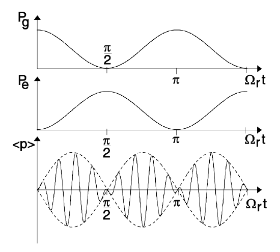
The coherent external field drives the population of the atomic system between the two available states with a period \(T_r = \pi/\Omega_r\). Applying the field only over half of this period leads to a complete inversion of the population. These Rabi-oscillations have been observed in various systems ranging from gases to semiconductors. Interestingly, the light emitted from the coherently driven two-level atom is not identical in frequency to the driving field. If we look at the Fourier spectrum of the polarization according to Eq.(\(\ref{eq2.3.56}\)), we obtain lines at frequencies \(\omega_{\pm} = \omega_{eg} \pm 2 \Omega_r\). This is clearly a nonlinear output and the sidebands are called Mollow-sidebands [2] . Most important for the existence of these oscillations is the coherence of the atomic system over at least one Rabi-oscillation. If this coherence is destroyed fast enough, the Rabi-oscillations cannot happen and it is then impossible to generate inversion in a two-level system by interaction with light. This is the case for a large class of situations in light-matter interaction. So we are interested what happens in the case of loss of coherence due to additional interaction of the atoms with a heat bath.
Density Operator
To study incoherent or dissipative processes it is useful to switch to a sta- tistical description using the density operator instead of deterministic wave functions similar to classical statistical mechanics, where the deterministic trajectories of particles are replaced by probability distributions.
The density operator of a pure state is defined by the dyadic product of the state with itself
\[\rho = |\psi \rangle \langle \psi| \nonumber \]
or in coordinate representation by a \(2 \times 2\)−matrix
\[\rho = \left ( \begin{matrix} \rho_{ee} & \rho_{eg} \\ \rho_{ge} & \rho_{gg} \end{matrix} \right ). \nonumber \]
In case of a pure state (\(\ref{eq2.3.9}\)) this is
\[\rho = \left ( \begin{matrix} c_ec_e^* & c_ec_g^* \\ c_gc_e^* & c_gc_g^* \end{matrix} \right ). \nonumber \]
It is obvious, that, for the rather simple case of a two-level system, each element of the density matrix corresponds to a physical quantity. The main diagonal contains the population probabilities for the levels and the off-diagonal element is the expectation value of the positive or negative frequency component of the dipole moment of the atom, i.e. its contribution to the medium polarization.
The expectation value of an arbitrary operator \(A\) can be computed using the trace formula
\[\langle A \rangle = Tr\{\rho A\} =\langle \psi |A| \psi \rangle . \nonumber \]
The advantage of the density operator is, that mixtures of pure states can also be treated in a statistical sense. For example, if the atom is in state \(|e \rangle \) with probability \(p_e\) and in state \(|g \rangle \) with probability \(p_g\) a density operator
\[\rho = p_e|e\rangle \langle e|+p_g|g\rangle \langle g| \nonumber \]
is defined, which can be used to compute the average values of observables in the proper statistical sense
\[\langle A\rangle =T_r \{\rho A\} = p_e\langle e|A|e\rangle +p_g \langle g|A|g\rangle . \nonumber \]
Since the matrices (\(\ref{eq2.3.27}\)) to (\(\ref{eq2.3.30}\)) build a complete base in the space of \(2 \times 2\)−matrices, we can express the density matrix as
\[\rho = \rho_{ee} \dfrac{1}{2} (1 + \sigma_z) + \rho_{gg} \dfrac{1}{2} (1 - \sigma_z) + \rho_{eg} \sigma^+ + \rho_{ge} \sigma^- \nonumber \]
\[=\dfrac{1}{2} 1 + \dfrac{1}{2} (\rho_{ee} -\rho_{gg}) \sigma_z + \rho_{eg} \sigma^+ + \rho_{ge} \sigma^-, \nonumber \]
since the trace of the density matrix is always one (normalization). Choosing the new base \(1, \sigma_x, \sigma_y, \sigma_z\), we obtain
\[\rho = \dfrac{1}{2} 1 + \dfrac{1}{2} (\rho_{ee} - \rho_{gg})\sigma_z + d_x \sigma_x + d_y \sigma_y, \nonumber \]
with
\[d_x = \dfrac{1}{2} (\rho_{eg} + \rho_{ge}) = \Re\{\langle \sigma^{(+)} \rangle \}, \nonumber \]
\[d_y = \dfrac{j}{2} (\rho_{eg} - \rho_{ge}) = \Im\{\langle \sigma^{(+)} \rangle \}, \nonumber \]
The expectation value of the dipole operator is given by (\(\ref{eq2.3.36}\))
\[\langle \vec{P}\rangle =T_r \{\rho \vec{P}\} = -\vec{M}^* Tr\{\rho \sigma^+\} + c.c. = -\vec{M}^* \rho_{ge} + c.c. \nonumber \]
From the Schrödinger equation for the wave function \(|\psi \rangle \) we can easily derive the equation of motion for the density operator, called the von Neumann equation
\[\dot{\rho} = \dfrac{d}{dt} |\psi \rangle \langle \psi| + h.c. = \dfrac{1}{j\hbar} H|\psi \rangle \langle \psi| - \dfrac{1}{j\hbar} |\psi \rangle \langle \psi| H = \dfrac{1}{j\hbar} [H, \rho]. \nonumber \]
Due to the linear nature of the equation, this is also the correct equation for a density operator describing an arbitrary mixture of states. In case of a two-level atom, the von Neumann equation is
\[\dot{\rho} = \dfrac{1}{j\hbar} [H_A, \rho] = -j \dfrac{\omega_{\in g}}{2} [\sigma_z, \rho]. \nonumber \]
Using the commutator relations (\(\ref{eq2.3.16}\)) - (\(\ref{eq2.3.18}\)), the result is
\[\dot{\rho}_{\in e} = 0,\label{eq2.3.71} \]
\[\dot{\rho}_{gg} = 0, \nonumber \]
\[\dot{\rho}_{eg} = -j \omega_{eg} \rho_{eg} \to \rho_{eg} (t) = e^{-j \omega_{eg} t} \rho_{eg} (0), \nonumber \]
\[\dot{\rho}_{ge} = j \omega_{eg} \rho_{ge} \to \rho_{ge} (t) = e^{j \omega_{eg} t} \rho_{ge} (0).\label{eq2.3.74} \]
Again the isolated two-level atom has a rather simple dynamics, the populations are constant, only the dipole moment oscillates with the transition frequency \(\omega_{\in g}\), if there has been a dipole moment induced at \(t = 0\), i.e. the system is in a superposition state.
Energy- and Phase-Relaxation
In reality, there is no isolated atom. Indeed in our case we are interested with a radiating atom, i.e. it has a dipole interaction with the field. The coupling with the infinitely many modes of the free field leads already to spontaneous emission, an irreversible process. We could treat this process by using the Hamiltonian
\[H = H_A + H_F + H_{A-F}. \nonumber \]
Here, \(H_A\) is the Hamiltonian of the atom, HF of the free field and \(H_{A-F}\) describes the interaction between them. A complete treatment along these lines is beyond the scope of this class and is usually done in classes on Quantum Mechanics. But the result of this calculation is simple and leads in the von Neumann equation of the reduced density matrix, i.e. the density matrix of the atom. With the spontaneous emission rate \(1/\tau_{sp}\),i.e. the inverse spontaneous life time \(\tau_{sp}\), the populations change according to
\[\dfrac{d}{dt} |c_e (t)|^2 = \dfrac{d}{dt} \rho_{ee} = -\Gamma_e \rho_{ee} + \Gamma_a \rho_{gg} \nonumber \]
with the abbreviations
\[\Gamma_e = \dfrac{1}{\tau_{sp}} (n_{th} + 1), \nonumber \]
\[\Gamma_a = \dfrac{1}{\tau_{sp}} n_{th}.\label{eq2.3.78} \]
Here, \(n_{th}\) is the number of thermally excited photons in the modes of the free field with frequency \(\omega_{eg}\), \(n_{th} = 1/(\exp (h\omega_{eg} /kT) - 1)\), at temperature \(T\).
The total probability of being in excited or ground state has to be maintained, that is
\[\dfrac{d}{dt} \rho_{gg} = -\dfrac{d}{dt} \rho_{ee} = \Gamma_e \rho_{ee} - \Gamma_a \rho_{gg}.\label{eq2.3.79} \]
If the populations decay, so does the polarization too, since \(\rho_{ge} = c_e^* c_g\), i.e.
\[\dfrac{d}{dt} \rho_{ge} j \omega_{eg} \rho_{eg} - \dfrac{\Gamma_e + \Gamma_a}{2} \rho_{ge}.\label{eq2.3.80} \]
Thus absorption as well as emission processes are also destructive to the phase, therefore, the corresponding rates add up in the phase decay rate.
Taking the coherent (\(\ref{eq2.3.71}\)-\(\ref{eq2.3.74}\)) and incoherent processes (\(\ref{eq2.3.79}\)-\(\ref{eq2.3.80}\)) into account results in the following equations for the normalized average dipole moment \(d = d_x + jd_y\) and the inversion \(w\)
\[\dot{d} = \dot{\rho}_{ge} = (j \omega_{eg} - \dfrac{1}{T_2})d,\label{eq2.3.81} \]
\[\dot{\omega} = \dot{\rho}_{ee} - \dot{\rho}_{gg} = \dfrac{\omega - \omega_0}{T_1},\label{eq2.3.82} \]
with the time constants
\[\dfrac{1}{T_1} = \dfrac{2}{T_2} = \Gamma_e + \Gamma_a = \dfrac{2n_{th} + 1}{\tau_{sp}} \nonumber \]
and equilibrium inversion \(w_0\), due to the thermal excitation of the atom by the thermal field
\[w_0 = \dfrac{\Gamma_a - \Gamma_e}{\Gamma_a + \Gamma_e} = \dfrac{-1}{1 + 2n_{th}} = -\tanh \left (\dfrac{\hbar\omega_{eg}}{2kT} \right ).\label{eq2.3.84} \]
The time constant \(T_1\) denotes the energy relaxation in the two-level system and \(T_2\) the phase relaxation. \(T_2\) is the correlation time between amplitudes \(c_e\) and \(c_g\). This coherence is destroyed by the interaction of the two-level system with the environment. In this model the energy relaxation is half the phase relaxation rate or
\[T_2 = 2T_1 \nonumber \]
The atoms in a laser medium do not only interact with the electromagnetic field, but in addition also with phonons of the host lattice, they might collide with each other in a gas laser and so on. All these processes must be considered when determining the energy and phase relaxation rates. Some of these processes are only destroying the phase, but do actually not lead to an energy loss in the system. Therefore, these processes reduce \(T_2\) but have no influence on \(T_1\). In real systems the phase relaxation time is most often much shorter than twice the energy relaxation time,
\[T_2 \le 2 T_1. \nonumber \]
If the inversion deviates from its equilibrium value \(w_0\) it relaxes back into equilibrium with a time constant \(T_1\). Equation (\(\ref{eq2.3.84}\)) shows that for all temperatures \(T \rangle 0\) the inversion is negative, i.e. the lower level is stronger populated than the upper level. Thus with incoherent thermal light inversion in a two-level system cannot be achieved. Inversion can only be achieved by pumping with incoherent light, if there are more levels and subsequent relaxation processes into the upper laser level. Due to these relaxation processes the rate \(\Gamma_a\) deviates from the equilibrium expression (\(\ref{eq2.3.78}\)), and it has to be replaced by the pump rate \(\Lambda\). If the pump rate \(\Lambda\) exceeds \(\Gamma_e\), the inversion corresponding to Equation (\(\ref{eq2.3.84}\)) becomes positive,
\[w_0 = \dfrac{\Lambda - \Gamma_e}{\Lambda + \Gamma_e}. \nonumber \]
If we allow for artificial negative temperatures, we obtain with \(T \langle 0\) for the ratio of relaxation rates
\[\dfrac{\Gamma_e}{\Gamma_a} = \dfrac{1+\bar{n}}{\bar{n}} = e^{\tfrac{\hbar \omega_{eg}}{kT}} \langle 1. \nonumber \]
Thus the pumping of the two-level system drives the system far away from thermal equilibrium, which has to be expected.
Two-Level Atom with a Coherent Classical External Field
If there is in addition to the coupling to an external heat bath, which models the spontaneous decay, pumping, and other incoherent processes, a coherent external field, the Hamiltonian has to be extended by the dipole interaction with that field,
\[H_E = -\vec{P} \vec{E} (\vec{x}_A, t). \nonumber \]
Again we use the interaction Hamiltonian in RWA
\[H_E = \dfrac{1}{2} \vec{M}^* \vec{E} (t)^{(-)} \sigma^+ + h.c.. \nonumber \]
This leads in the von Neumann equation to the additional term
\[\dot{\rho} |_E = \dfrac{1}{j\hbar} [H_E, \rho] \nonumber \]
\[= \dfrac{1}{2j\hbar} \vec{M}^* \vec{E} (t)^{(-)} [\sigma^+, \rho] + h.c. \nonumber \]
or
\[\rho{\rho}_{ee}|_E = \dfrac{1}{2j\hbar} \vec{E}^{(-)} \rho_{ge} + c.c., \nonumber \]
\[\rho{\rho}_{ge}|_E = \dfrac{1}{2j\hbar} \vec{E}^{(+)} (\rho_{ee} -\rho_{gg}), \nonumber \]
\[\rho{\rho}_{gg}|_E = -\dfrac{1}{2j\hbar} \vec{E}^{(-)} \rho_{ge} + c.c., \nonumber \]
The evolution of the dipole moment and the inversion is changed by
\[\dot{d}|_E = \dot{\rho}_{ge}|_E = \dfrac{1}{2j\hbar} \vec{M} \vec{E}^{(+)} w, \nonumber \]
\[\dot{w}|_E = \dot{\rho}_{ee}|_E - \dot{\rho}_{gg}|_E = \dfrac{1}{j\hbar} (\vec{M}^* \vec{E}^{(-)} d^* - \vec{M} \vec{E}^{(+)} d). \nonumber \]
Thus, the total dynamics of the two-level system including the pumping and dephasing processes from Eqs.(\(\ref{eq2.3.81}\)) and (\(\ref{eq2.3.82}\)) is given by
\[\dot{d} = -(\dfrac{1}{T_2} - j \omega_{eg})d + \dfrac{1}{2j \hbar} \vec{M} \vec{E}^{(+)} w, \nonumber \]
\[\dot{w} = -\dfrac{w-w_0}{T_1} + \dfrac{1}{j\hbar} (\vec{M}^* \vec{E}^{(-)} d - \vec{M} \vec{E}^{(+)} d^*). \nonumber \]
These equations are called Bloch-equations. They describe the dynamics of an atom interacting with a classical electric field. Together with Equation (2.2.2) they build the Maxwell-Bloch equations.