
2.4: Dielectric Susceptibility
- Page ID
- 48236
\( \newcommand{\vecs}[1]{\overset { \scriptstyle \rightharpoonup} {\mathbf{#1}} } \)
\( \newcommand{\vecd}[1]{\overset{-\!-\!\rightharpoonup}{\vphantom{a}\smash {#1}}} \)
\( \newcommand{\dsum}{\displaystyle\sum\limits} \)
\( \newcommand{\dint}{\displaystyle\int\limits} \)
\( \newcommand{\dlim}{\displaystyle\lim\limits} \)
\( \newcommand{\id}{\mathrm{id}}\) \( \newcommand{\Span}{\mathrm{span}}\)
( \newcommand{\kernel}{\mathrm{null}\,}\) \( \newcommand{\range}{\mathrm{range}\,}\)
\( \newcommand{\RealPart}{\mathrm{Re}}\) \( \newcommand{\ImaginaryPart}{\mathrm{Im}}\)
\( \newcommand{\Argument}{\mathrm{Arg}}\) \( \newcommand{\norm}[1]{\| #1 \|}\)
\( \newcommand{\inner}[2]{\langle #1, #2 \rangle}\)
\( \newcommand{\Span}{\mathrm{span}}\)
\( \newcommand{\id}{\mathrm{id}}\)
\( \newcommand{\Span}{\mathrm{span}}\)
\( \newcommand{\kernel}{\mathrm{null}\,}\)
\( \newcommand{\range}{\mathrm{range}\,}\)
\( \newcommand{\RealPart}{\mathrm{Re}}\)
\( \newcommand{\ImaginaryPart}{\mathrm{Im}}\)
\( \newcommand{\Argument}{\mathrm{Arg}}\)
\( \newcommand{\norm}[1]{\| #1 \|}\)
\( \newcommand{\inner}[2]{\langle #1, #2 \rangle}\)
\( \newcommand{\Span}{\mathrm{span}}\) \( \newcommand{\AA}{\unicode[.8,0]{x212B}}\)
\( \newcommand{\vectorA}[1]{\vec{#1}} % arrow\)
\( \newcommand{\vectorAt}[1]{\vec{\text{#1}}} % arrow\)
\( \newcommand{\vectorB}[1]{\overset { \scriptstyle \rightharpoonup} {\mathbf{#1}} } \)
\( \newcommand{\vectorC}[1]{\textbf{#1}} \)
\( \newcommand{\vectorD}[1]{\overrightarrow{#1}} \)
\( \newcommand{\vectorDt}[1]{\overrightarrow{\text{#1}}} \)
\( \newcommand{\vectE}[1]{\overset{-\!-\!\rightharpoonup}{\vphantom{a}\smash{\mathbf {#1}}}} \)
\( \newcommand{\vecs}[1]{\overset { \scriptstyle \rightharpoonup} {\mathbf{#1}} } \)
\(\newcommand{\longvect}{\overrightarrow}\)
\( \newcommand{\vecd}[1]{\overset{-\!-\!\rightharpoonup}{\vphantom{a}\smash {#1}}} \)
\(\newcommand{\avec}{\mathbf a}\) \(\newcommand{\bvec}{\mathbf b}\) \(\newcommand{\cvec}{\mathbf c}\) \(\newcommand{\dvec}{\mathbf d}\) \(\newcommand{\dtil}{\widetilde{\mathbf d}}\) \(\newcommand{\evec}{\mathbf e}\) \(\newcommand{\fvec}{\mathbf f}\) \(\newcommand{\nvec}{\mathbf n}\) \(\newcommand{\pvec}{\mathbf p}\) \(\newcommand{\qvec}{\mathbf q}\) \(\newcommand{\svec}{\mathbf s}\) \(\newcommand{\tvec}{\mathbf t}\) \(\newcommand{\uvec}{\mathbf u}\) \(\newcommand{\vvec}{\mathbf v}\) \(\newcommand{\wvec}{\mathbf w}\) \(\newcommand{\xvec}{\mathbf x}\) \(\newcommand{\yvec}{\mathbf y}\) \(\newcommand{\zvec}{\mathbf z}\) \(\newcommand{\rvec}{\mathbf r}\) \(\newcommand{\mvec}{\mathbf m}\) \(\newcommand{\zerovec}{\mathbf 0}\) \(\newcommand{\onevec}{\mathbf 1}\) \(\newcommand{\real}{\mathbb R}\) \(\newcommand{\twovec}[2]{\left[\begin{array}{r}#1 \\ #2 \end{array}\right]}\) \(\newcommand{\ctwovec}[2]{\left[\begin{array}{c}#1 \\ #2 \end{array}\right]}\) \(\newcommand{\threevec}[3]{\left[\begin{array}{r}#1 \\ #2 \\ #3 \end{array}\right]}\) \(\newcommand{\cthreevec}[3]{\left[\begin{array}{c}#1 \\ #2 \\ #3 \end{array}\right]}\) \(\newcommand{\fourvec}[4]{\left[\begin{array}{r}#1 \\ #2 \\ #3 \\ #4 \end{array}\right]}\) \(\newcommand{\cfourvec}[4]{\left[\begin{array}{c}#1 \\ #2 \\ #3 \\ #4 \end{array}\right]}\) \(\newcommand{\fivevec}[5]{\left[\begin{array}{r}#1 \\ #2 \\ #3 \\ #4 \\ #5 \\ \end{array}\right]}\) \(\newcommand{\cfivevec}[5]{\left[\begin{array}{c}#1 \\ #2 \\ #3 \\ #4 \\ #5 \\ \end{array}\right]}\) \(\newcommand{\mattwo}[4]{\left[\begin{array}{rr}#1 \amp #2 \\ #3 \amp #4 \\ \end{array}\right]}\) \(\newcommand{\laspan}[1]{\text{Span}\{#1\}}\) \(\newcommand{\bcal}{\cal B}\) \(\newcommand{\ccal}{\cal C}\) \(\newcommand{\scal}{\cal S}\) \(\newcommand{\wcal}{\cal W}\) \(\newcommand{\ecal}{\cal E}\) \(\newcommand{\coords}[2]{\left\{#1\right\}_{#2}}\) \(\newcommand{\gray}[1]{\color{gray}{#1}}\) \(\newcommand{\lgray}[1]{\color{lightgray}{#1}}\) \(\newcommand{\rank}{\operatorname{rank}}\) \(\newcommand{\row}{\text{Row}}\) \(\newcommand{\col}{\text{Col}}\) \(\renewcommand{\row}{\text{Row}}\) \(\newcommand{\nul}{\text{Nul}}\) \(\newcommand{\var}{\text{Var}}\) \(\newcommand{\corr}{\text{corr}}\) \(\newcommand{\len}[1]{\left|#1\right|}\) \(\newcommand{\bbar}{\overline{\bvec}}\) \(\newcommand{\bhat}{\widehat{\bvec}}\) \(\newcommand{\bperp}{\bvec^\perp}\) \(\newcommand{\xhat}{\widehat{\xvec}}\) \(\newcommand{\vhat}{\widehat{\vvec}}\) \(\newcommand{\uhat}{\widehat{\uvec}}\) \(\newcommand{\what}{\widehat{\wvec}}\) \(\newcommand{\Sighat}{\widehat{\Sigma}}\) \(\newcommand{\lt}{<}\) \(\newcommand{\gt}{>}\) \(\newcommand{\amp}{&}\) \(\definecolor{fillinmathshade}{gray}{0.9}\)If the incident field is monofrequent, i.e.
\[\vec{E} (t)^{(+)} = \hat{\vec{E}} e^{i\omega t},\label{eq2.4.1} \]
and assuming that the inversion \(w\) of the atom will be well represented by its time average \(w_s\), then the dipole moment will oscillate with the same frequency in the stationary state
\[d = \hat{d} e^{i\omega t},\label{eq2.4.2} \]
and the inversion will adjust to a new stationary value \(w_s\). With ansatz (\(\ref{eq2.4.1}\)) and (\(\ref{eq2.4.2}\)) in Eqs. (2.3.98) and (2.3.99), we obtain
\[\hat{d} = \dfrac{-j}{2\hbar} \dfrac{w_s}{1/T_2 + j(\omega - \omega_{eg})} \vec{M} \hat{\vec{E}},\label{eq2.4.3} \]
\[w_s = \dfrac{w_0}{1 + \tfrac{T_1}{\hbar^2} \tfrac{1/T_2 |\vec{M} \hat{\vec{E}}|^2}{(1/T_2)^2 + (\omega_{eg} - \omega)^2}}. \nonumber \]
We introduce the normalized lineshape function, which is in this case a Lorentzian,
\[L(\omega) = \dfrac{(1/T_2)^2}{(1/T_2)^2 + (\omega_{eg} - \omega)^2}, \nonumber \]
and connect the square of the field \(|\hat{\vec{E}}|^2\) to the intensity \(I\) of a propagating plane wave, according to Equation (2.2.27), \(I = \dfrac{1}{2Z_F} |\hat{\vec{E}}|^2\),
\[w_s = \dfrac{w_0}{1 + \tfrac{I}{I_s} L(\omega)}. \nonumber \]
Thus the stationary inversion depends on the intensity of the incident light, therefore, \(w_0\) can be called the unsaturated inversion, \(w_s\) the saturated inversion and \(I_s\), with
\[I_s = \left [ \dfrac{2T_1T_2 Z_F}{\hbar^2} \dfrac{|\vec{M} \hat{\vec{E}}|^2}{|\hat{\vec{E}}|^2} \right ]^{-1}, \nonumber \]
is the saturation intensity. The expectation value of the dipole operator is then given by
\[<\vec{p}>= -(\vec{M}^* d + \vec{M} d^*). \nonumber \]
Multiplication with the number of atoms per unit volume \(N\) relates the dipole moment of the atom to the complex polarization \(\hat{\vec{P}}^+\) of the medium, and therefore to the susceptibility according to
\[\hat{\vec{P}}^{(+)} = -2N \vec{M}^* \hat{d},\label{eq2.4.9} \]
\[\hat{\vec{P}}^{(+)} = \epsilon_x \chi (\omega) \hat{\vec{E}}.\label{eq2.4.10} \]
From the definitions (\(\ref{eq2.4.9}\)), (\(\ref{eq2.4.10}\)) and Equation (\(\ref{eq2.4.2}\)) we obtain for the linear susceptibility of the medium
\[\chi (\omega) = \vec{M}^* \vec{M}^T \dfrac{jN}{\hbar \epsilon_0} \dfrac{w_s}{1/T_2 + j(\omega - \omega_{eg})}. \nonumber \]
which is a tensor. In the following we assume that the direction of the atom is random, i.e. the alignment of the atomic dipole moment \(\vec{M}\) and the electric field is random. Therefore, we have to average over the angle enclosed between the electric field of the wave and the atomic dipole moment, which results in
\[\overline{\left (\begin{matrix} M_x M_x & M_x M_y & M_x M_z \\ M_y M_x & M_y M_y & M_y M_z \\ M_z M_x & M_z M_y & M_z M_z \end{matrix} \right )} = \left (\begin{matrix} \overline{M_x^2} & 0 & 0 \\ 0 & \overline{M_y^2} & 0 \\ 0 & 0 & \overline{M_y^2} \end{matrix} \right ) = \dfrac{1}{3} |\vec{M}|^2 1. \nonumber \]
Thus, for homogeneous and isotropic media the susceptibility tensor shrinks to a scalar
\[\chi (\omega) = \dfrac{1}{3} |\vec{M}|^2 \dfrac{jN}{\hbar \epsilon_0} \dfrac{w_s}{1/T_2 + j (\omega - \omega_{eg})}. \nonumber \]
Real and imaginary part of the susceptibility
\[\chi (\omega) = \chi ' (\omega) + j \chi '' (\omega) \nonumber \]
are then given by
\[\chi '(\omega) = -\dfrac{|\vec{M}|^2 N w_s T_2^2 (\omega_{eg} - \omega)}{3\hbar \epsilon_0} L(\omega), \nonumber \]
\[\chi '' (\omega) = \dfrac{|\vec{M}|^2 N w_s T_s}{3 \hbar \epsilon_0} L(\omega). \nonumber \]
If the incident radiation is weak enough, i.e.
\[T_1 T_2 \dfrac{|\vec{M}^* \hat{\vec{E}}|^2}{\hbar^2} L(\omega) \ll 1 \nonumber \]
we obtain \(w_s \approx w_0\). Since \(w_0 < 0\), and especially for optical transitions \(w_0 = -1\), real and imaginary part of the susceptibility are shown in Figure 2.4.
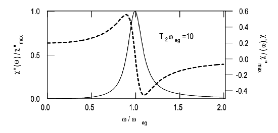
The susceptibility computed quantum mechanically compares well with the classical susceptibility derived from the harmonic oscillator model close to the transistion frequency for a transition with reasonably high \(Q = T_2\omega_{ab}\). Note, there is an appreciable deviation far away from resonance. Far off resonance the rotating wave approximation should not be used.
The physical meaning of the real and imaginary part of the susceptibility becomes obvious, when the propagation of a plane electro-magnetic wave through this medium is considered,
\[\vec{E} (z, t) = \Re \{ \hat{\vec{E}} e^{j(\omega t - kz)} \}, \nonumber \]
which is propagating in the positive \(z\)-direction. The propagation constant \(k\) is related to the susceptibility by
\[k = \omega \sqrt{\mu_0 \epsilon_0 (1 + \chi (\omega))} \approx k_0 \left (1 + \dfrac{1}{2} \chi (\omega) \right ), \text{ with } k_0 = \omega \sqrt{\mu_0 \epsilon_0} \nonumber \]
for \(|\chi| \ll 1\). Under this assumption we obtain
\[k = k_0 (1 + \dfrac{\chi '}{2} ) + j k_0 \dfrac{\chi ''}{2}. \nonumber \]
The real part of the susceptibility contributes to the refractive index \(n = 1 + \chi '/2\). In case of \(\chi '' < 0\), the imaginary part leads to an exponential damping of the wave. For \(\chi '' > 0\) amplification takes place. Amplification of the wave is possible for \(w_0 > 0\), i.e. an inverted medium.
The phase relaxation rate \(1/T_2\) of the dipole moment determines the width of the absorption line or the bandwidth of the amplifier.