
2.8: Pulse Shapes and Time-Bandwidth Products
- Page ID
- 48948

The following table 2.2 shows pulse shape, spectrum and time bandwidth products of some often used pulse forms.
| \(a(t)\) | \(\hat{a} (\omega) = \int_{-\infty}^{\infty} a(t) e^{-j\omega t} dt\) | \(\Delta t\) | \(\Delta t \cdot \Delta f\) |
|---|---|---|---|
| Gauss: \(e^{-\tfrac{t^2}{t\tau^2}}\) | \(\sqrt{2\pi} \tau e^{-\tfrac{1}{t} \tau^2 \omega^2}\) | \(2\sqrt{\ln 2} \tau\) | 0.441 |
|
Hyperbolicsecant: sech (\(\dfrac{t}{\tau}\)) |
\(\dfrac{\tau}{2}\) sech (\(\dfrac{\pi}{2} \tau \omega\)) | \(1.7627 \tau\) | 0.315 |
| Rect-function: \(= \begin{cases} 1, |t| \le \tau/2 \\ 0, |t| > \tau/2 \end{cases}\) |
\(\tau \dfrac{\sin (\tau \omega/2)}{\tau \omega/2}\) | \(\tau\) | 0.886 |
| Lorentzian: \(\dfrac{1}{1 + (t/\tau)^2\) | \(2\pi \tau e^{-|\tau \omega|}\) | \(1.287 \tau\) | 0.142 |
| Double-Exponential: \(e^{-|\tfrac{t}{\tau}|}\) | \(\dfrac{\tau}{1 + (\omega \tau)^2}\) | \(\ln 2 \tau\) | 0.142 |
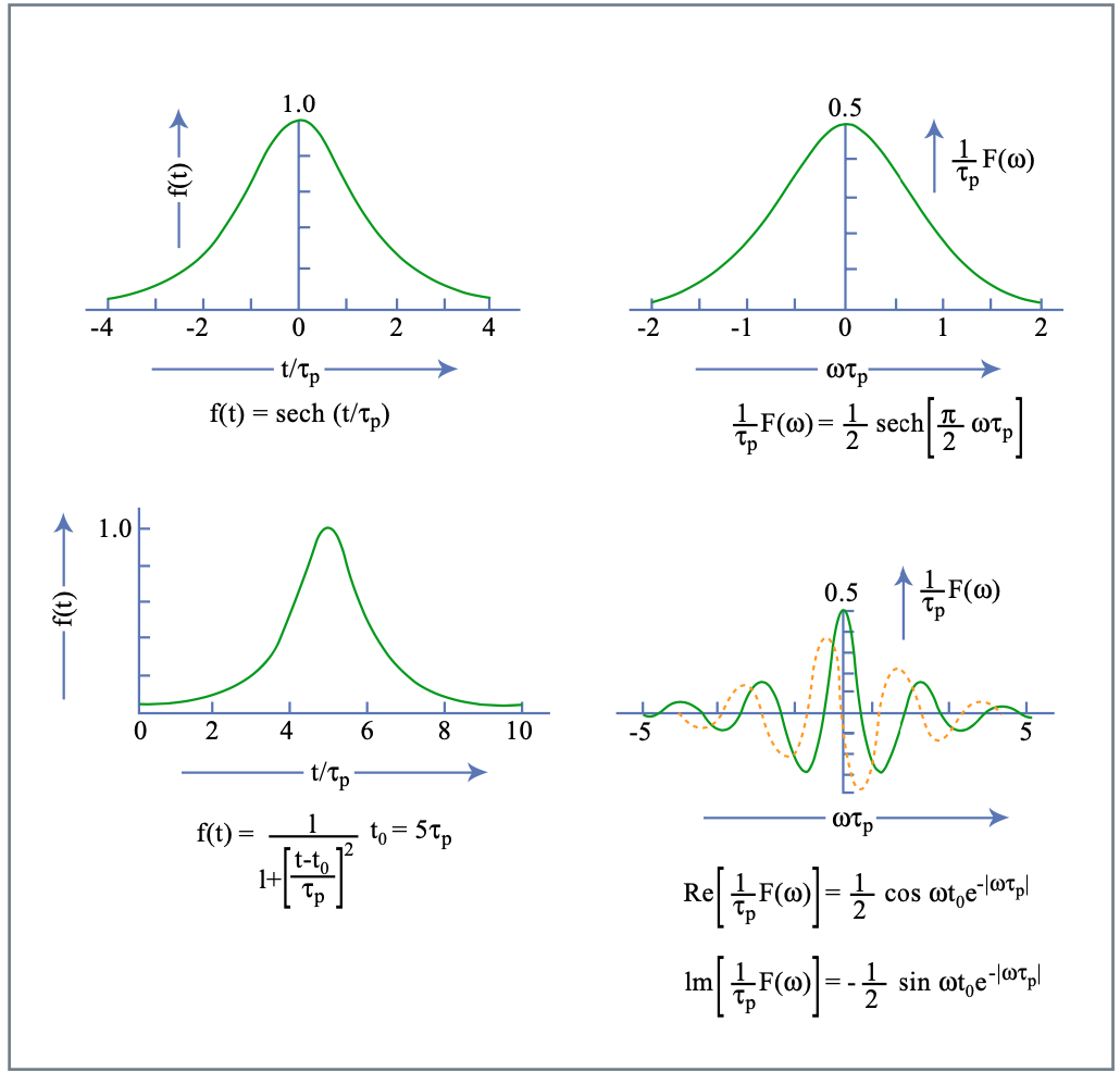
Figure 2.14: Fourier relationship to table above.
Figure by MIT OCW.
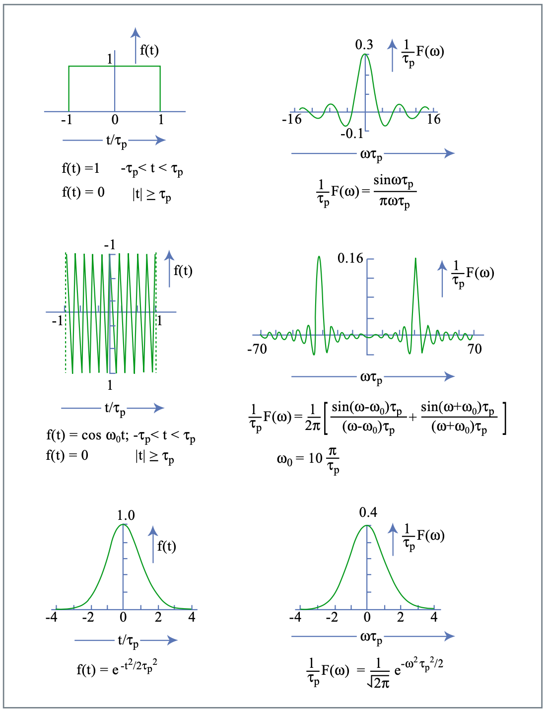
Figure 2.15: Fourier relationships to table above. Figure by MIT OCW.
Bibliography
[1] I. I. Rabi: "Space Quantization in a Gyrating Magnetic Field,". Phys. Rev. 51, 652-654 (1937).
[2] B. R. Mollow, "Power Spectrum of Light Scattered by Two-Level Sys- tems," Phys. Rev 188, 1969-1975 (1969).
[3] P. Meystre, M. Sargent III: Elements of Quantum Optics, Springer Verlag (1990).
[4] L. Allen and J. H. Eberly: Optical Resonance and Two-Level Atoms, Dover Verlag (1987).
[5] G. B. Whitham: "Linear and Nonlinear Waves," John Wiley and Sons, NY (1973).