2.7: Kramers-Kroenig Relations

The linear susceptibility is the frequency response of a linear system to an applied electric field, which is causal, and therefore real and imaginary parts obey Kramers-Kroenig Relations

\[\chi_r (\Omega) = \dfrac{2}{\pi} \int_{0}^{\infty} \dfrac{\omega \chi_i (\omega)}{\omega^2 - \Omega^2} d\omega = n^2 (\Omega) - 1, \nonumber \]

\[\chi_i (\Omega) = -\dfrac{2}{\pi} \int_{0}^{\infty} \dfrac{\Omega \chi_r (\omega)}{\omega^2 - \Omega^2} d\omega. \nonumber \]

In transparent media one is operating far away from resonances. Then the absorption or imaginary part of the susceptibility can be approximated by

\[\chi_i (\Omega) = \sum_i A_i \delta (\omega -\omega_i) \nonumber \]

and the Kramers-Kroenig relation results in a Sellmeier Equation for the refractive index

\[\begin{align*} n^2 (\Omega) &= 1 + \sum_i A_i \dfrac{\omega_i}{\omega_i^2 - \Omega^2} \\[4pt] &= 1 + \sum_i a_i \dfrac{\lambda}{\lambda^2 - \lambda_i^2} \end{align*} \nonumber \]

For an example Table 2.1 shows the sellmeier coefficients for fused quartz and sapphire.

Table 2.1: Table with Sellmeier coefficients for fused quartz and sapphire.

	Fused Quartz	Sapphire
\(a_1\)	0.6961663	1.023798
\(a_2\)	0.4079426	1.058364
\(a_3\)	0.8974794	5.280792
\(\lambda_1^2\)	\(4.679148 \cdot 10^{-3}\)	\(3.77588 \cdot 10^{-3}\)
\(\lambda_2^2\)	\(1.3512063 \cdot 10^{-2}\)	\(1.22544 \cdot 10^{-2}\)
\(\lambda_3^2\)	\(0.9793400 \cdot 10^{2}\)	\(3.213616 \cdot 10^{2}\)

A typical situation for a material having resonances in the UV and IR, such as glass, is shown in Figure 2.12

Figure 2.12: Typcial distribution of absorption lines in a medium transparent in the visible. Figure by MIT OCW.

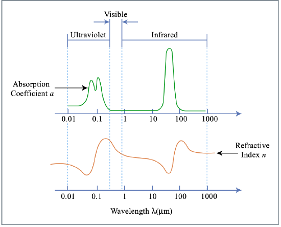
The regions where the refractive index is decreasing with wavelength is usually called normal dispersion range and the opposite behavior abnormal dispersion

\[\begin{array} {rcl} {\dfrac{dn}{d\lambda}} & < & {\text{0: normal dispersion (blue refracts more than red)}} \\ {\dfrac{dn}{d\lambda}} & > & {\text{0: abnormal dispersion}} \end{array}\nonumber \]

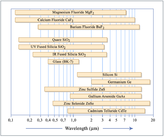
Fig.2.13 shows the transparency range of some often used media.

Figure 2.13: Transparency range of some materials. Figure by MIT OCW.