2.6: Pulse Propagation with Dispersion and Gain

In many cases, mode locking of lasers can be most easily studied in the time domain. Then mode locking becomes a nonlinear, dissipative wave propagation problem. In this chapter, we discuss the basic elements of pulse propagation in linear and nonlinear media, as far as it is necessary for the following chapters. A comprehensive discussion of nonlinear pulse propagation can be found in [6].

We consider the electric field of a monochromatic electromagnetic wave with frequency \(\Omega\), which propagates along the \(z\)-axis, and is polarized along the \(x\)-axis, (Figure 2.5).

Figure 2.5: Transverse electro-magnetic wave. Figure by MIT OCW.

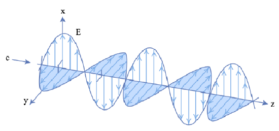
In a linear, isotropic, homogeneous, and lossless medium the electric field of that electromagnetic wave is given by

\[\begin{array} {rcl} {\vec{E} (z, t)} & = & {\vec{e}_x E(z, t),} \\ {E(z, t)} & = & {\Re \{\tilde{E} (\Omega) e^{j(\omega t - Kz)}\}} \\ {} & = & {|\tilde{E}| \cos (\Omega t - Kz + \phi),} \end{array} \nonumber \]

where \(\tilde{E} = |\tilde{E}|e^{j\phi}\) is the complex wave amplitude of the electromagnetic wave at frequency \(\Omega\) and wave number \(K = \Omega /c = n\Omega /c_0\). Here, \(n\) is the refractive index, \(c\) the velocity of light in the medium and \(c_0\) the velocity of light in vacuum, respectively. The planes of constant phase propagate with the phase velocity \(c\) of the wave. Usually, we have a superposition of many frequencies with spectrum shown in Figure 2.6

Figure 2.6: Electric field and pulse envelope in frequency domain.

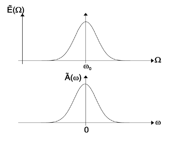
In general, the refractive index is a function of frequency and one is interested in the propagation of a pulse, that is produced by a superposition of monochromatic waves grouped around a certain carrier frequency \(\omega_0\) (Figure 2.6)

\[E(z, t) = \Re \left \{ \dfrac{1}{2\pi} \int_{0}^{\infty} \hat{E} (\Omega) e^{j(\Omega t - K(\Omega) z)} d \Omega \right \}.\label{eq2.6.2} \]

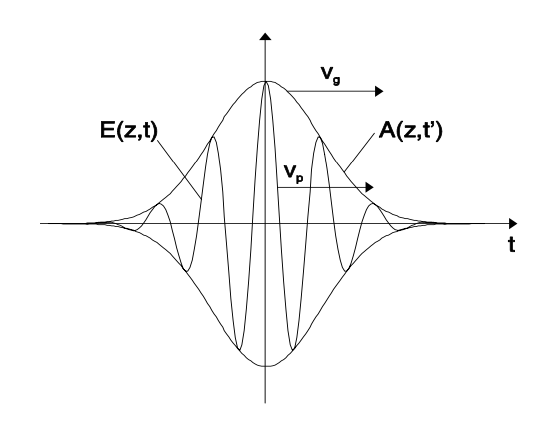
We can always separate the complex electric field in Equation (\(\ref{eq2.6.2}\)) into a carrier wave and an envelope \(A(z, t)\)

\[E(z, t) = \Re \{A(z, t) e^{j (\omega_0 t - K(\omega_0)z)} \}. \nonumber \]

The envelope is given by

\[A(z, t) = \dfrac{1}{2\pi} \int_{-\omega_0 \to -\infty}^{\infty} \tilde{A} (\omega) e^{j (\omega_0 t - K(\omega_0)z)} d\omega,\label{eq2.6.4} \]

where we introduced the offset frequency, offset wave vector and spectrum of the envelope (see Figure 2.7)

\[\omega = \Omega - \omega_0 \nonumber \]

\[k(\omega) = K(\omega_0 + \omega) - K(\omega_0), \nonumber \]

\[\tilde{A} (\omega) = \tilde{E} (\Omega = \omega_0 + \omega) \nonumber \]

Depending on the dispersion relation, the pulse will be reshaped during propagation.

Figure 2.7: Electric field and pulse envelope in time domain.

Dispersion

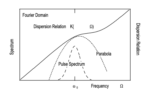
If the spectral width of the pulse is small compared to the carrier frequency, the envelope is only slowly varying with time. Additionally, if the dispersion relation \(k(\omega)\) is only slowly varying over the pulse spectrum, it is useful to represent the dispersion relation, \(K(\Omega)\),see Figure 2.8, by its Taylor expansion

\[k(\omega) = k'\omega + \dfrac{k''}{2} \omega^2 + \dfrac{k^(3)}{6} \omega^3 + O(\omega^4)\label{eq2.6.8} \]

If the refractive index depends on frequency, the dispersion relation is no longer linear with respect to frequency, see Figure 2.8.

Figure 2.8: Taylor expansion of dispersion relation.

For the moment, we keep only the first term, the linear term, in Eq.(\(\ref{eq2.6.8}\)). Then we obtain for the pulse envelope from (\(\ref{eq2.6.4}\)) by definition of the group velocity \(v_g = 1/k'\)

\[A (z, t) = A(0, t - z/v_g). \nonumber \]

Thus the derivative of the dispersion relation at the carrier frequency determines the velocity of the corresponding wave packet. We introduce the local time \(t' = t - z/v_g\). With respect to this local time the pulse shape is invariant during propagation

\[A(z, t') = A(0, t'). \nonumber \]

If the spectrum of the pulse becomes broad enough, so that the second order term in (Eq.(\(\ref{eq2.6.8}\))) becomes important, wave packets with different carrier frequencies propagate with different group velocities and the pulse spreads. When keeping in the dispersion relation terms up to second order it follows from (Eq.(\(\ref{eq2.6.4}\)))

\[\dfrac{\partial A(z, t')}{\partial z} = -j\dfrac{k''}{2} \dfrac{\partial^2 A(z, t')}{\partial t'^2}. \nonumber \]

This is equivalent to the Schrödinger equation for a nonrelativistic free particle. Like in Quantum Mechanics, it describes the spreading of a wave packet. Here, the spreading is due to the first nontrivial term in the dispersion relation, which describes spreading of an electromagnetic wave packet via group velocity dispersion (GVD). Of course, we can keep all terms in the dispersion relation, which would lead to higher order derivatives in the equation for the envelope.

\[\dfrac{\partial A(z, t')}{\partial z} = j \sum_{n = 2}^{\infty} \dfrac{k^{(n)}}{n!} \left ( j \dfrac{\partial}{\partial t'} \right )^n A(z, t').\label{eq2.6.12} \]

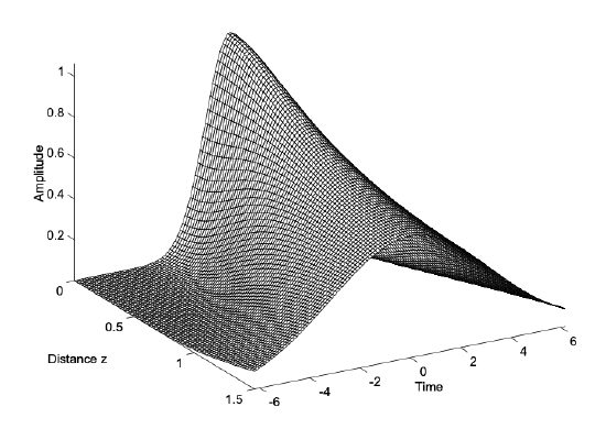
Therefore, one usually calls the first term dispersion and the higher order terms higher order dispersion. In the following, we always work in the local time frame to get rid of the trivial motion of the pulse. Therefore, we drop the prime to simplify notation. Figure 2.9 shows the evolution of a Gaussian wave packet during propagation in a medium which has no higher order dispersion and \(k'' = 2\) is given in normalized units. The pulse spreads continuously.

Figure 2.9: Amplitude of the envelope of a Gaussian pulse, \(|A(z, t')|\), in a dispersive medium.

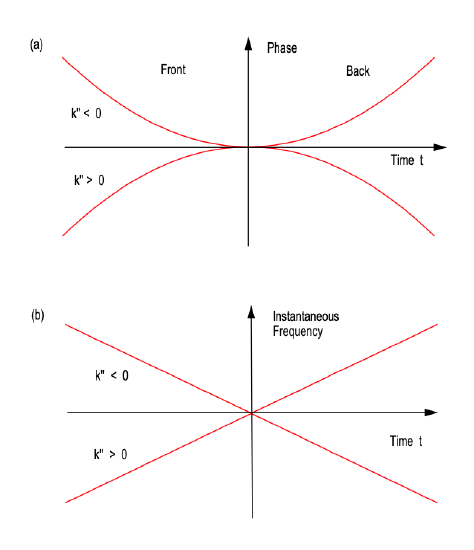
As shown in Figure 2.10(a), during propagation in the dispersive medium, the pulse acquires a linear chirp, i.e. its phase becomes parabolic. The derivative of the phase with respect to time is the instantaneous frequency Figure 2.10(b). It indicates, that the low frequencies are in the front of the pulse, whereas the high frequencies are in the back of the pulse. This is due to the positive dispersion \(k'' > 0\), which causes, that wave packets with lower frequencies travel faster than wave packets with higher frequencies.

Figure 2.10: (a) Phase and (b) instantaneous frequency of a Gaussian pulse during propagation through a medium with positive or negative dispersion.

Loss and Gain

If the medium considered has loss, we can incorporate this loss into a complex refractive index

\[n(\Omega) = n_r (\Omega) + jn_i (\Omega). \nonumber \]

The refractive index is determined by the linear response, \(\chi (\Omega)\), of the polarization in the medium onto the electric field induced in the medium

\[n(\Omega) = \sqrt{1 + \chi (\Omega)}. \nonumber \]

For an optically thin medium, i.e. \(|\chi (\Omega)| \ll 1\) we obtain approximately

\[n(\Omega) \approx 1 + \dfrac{\chi (\Omega)}{2}.\label{eq2.6.15} \]

For a two level atom with an electric dipole transition, the susceptibility is given, in the rotating wave approximation, by the complex Lorentzian lineshape

\[\chi (\Omega) = \dfrac{2j\alpha}{1 - j \tfrac{\Omega - \Omega_0}{\Delta \Omega}}. \nonumber \]

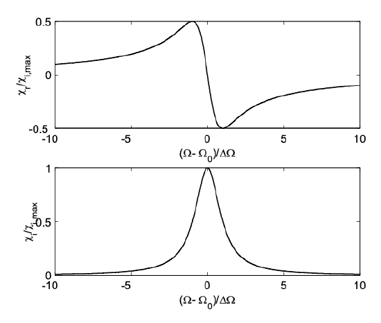
where \(\alpha\) will turn out to be the peak absorption or gain of the transition, which is proportional to the density of the atomic inversion, \(\Omega_0\) is the center frequency of the optical transition and \(\Delta \Omega\) is the HWHM linewidth of the transition. Figure 2.11 shows the normalized real and imaginary part of the complex Lorentzian

\[\chi_r (\Omega) = \dfrac{-2\alpha \tfrac{\Omega - \Omega_0}{\Delta \Omega}}{1 + (\tfrac{\Omega - \Omega_0}{\Delta \Omega})^2}, \nonumber \]

\[\chi_i (\Omega) = \dfrac{2 \alpha}{1 + (\tfrac{\Omega - \Omega_0}{\Delta \Omega})^2}, \nonumber \]

which are the real- and imaginary part of the complex susceptibility for a noninverted optical transition, i.e. loss.

Figure 2.11: Normalized real and imaginary part of the complex Lorentzian.

The real part of the transition modifies the real part of the refractive index of the medium, whereas the imaginary part leads to loss in the case of a noninverted medium.

In the derivation of the wave equation for the pulse envelope (\(\ref{eq2.6.12}\)) in section 2.6.1, there was no restriction to a real refractive index. Therefore, the wave equation (\(\ref{eq2.6.12}\)) also treats the case of a complex refractive index. If we assume a medium with the complex refractive index (\(\ref{eq2.6.15}\)), then the wave number is given by

\[K(\Omega) = \dfrac{\Omega}{c_0} \left ( 1 + \dfrac{1}{2} (\chi_r (\Omega) + j \chi_i (\Omega)) \right ).\label{eq2.6.19} \]

Since we introduced a complex wave number, we have to redefine the group velocity as the inverse derivative of the real part of the wave number with respect to frequency. At line center, we obtain

\[v_g^{-1} = \dfrac{\partial K_r (\Omega)}{\partial \Omega} |_{\Omega_0} = \dfrac{1}{c_0} \left (1 - \alpha \dfrac{\Omega_0}{\Delta \Omega}\right ). \nonumber \]

Thus, for a narrow absorption line, \(\alpha > 0\) and \(\tfrac{\Omega_0}{\Delta \Omega} \gg 1\), the absolute value of the group velocity can become much larger than the velocity of light in vacuum. The opposite is true for an inverted, and therefore, amplifying transition, \(\alpha < 0\). There is nothing wrong with it, since the group velocity only describes the motion of the peak of a Gaussian wave packet, which is not a causal wave packet. A causal wave packet is identical to zero for some earlier time \(t < t_0\), in some region of space. A Gaussian wave packet fills the whole space at any time and can be reconstructed by a Taylor expansion at any time. Therefore, the tachionic motion of the peak of such a signal does not contradict special relativity.

The imaginary part in the wave vector (\(\ref{eq2.6.19}\)), due to gain and loss, has to be completely treated in the envelope equation (\(\ref{eq2.6.12}\)). In the frequency domain this leads for a wave packet with a carrier frequency at line center, \(\omega_0 = \Omega_0\) and \(K_r (\Omega_0) = k_0\), to the term

\[\left.\dfrac{\partial \tilde{A} (z, \omega)}{\partial z} \right|_{(loss)} = \dfrac{-\alpha k_0}{1 + (\tfrac{\omega}{\Delta \Omega})^2} \tilde{A} (z, \omega). \nonumber \]

In the time domain, we obtain up to second order in the inverse linewidth

\[\left.\dfrac{\partial \tilde{A} (z, \omega)}{\partial z} \right|_{(loss)} = -\alpha k_0 \left (1 + \dfrac{1}{\Delta \Omega^2} \dfrac{\partial^2}{\partial t^2} \right ) A(z, t), \nonumber \]

which corresponds to a parabolic approximation of the Lorentzian line shape at line center, (Figure 2.11). For an inverted optical transition, we obtain a similar equation, we only have to replace the loss by gain

\[\left.\dfrac{\partial \tilde{A} (z, \omega)}{\partial z}\right|_{(gain)} = g \left (1 + \dfrac{1}{\Omega_g^2} \dfrac{\partial^2}{\partial t^2} \right ) A(z, t), \nonumber \]

where \(g = -\alpha k_0\) is the peak gain at line center per unit length and \(\Omega_g\) is the HWHM linewidth of the gain transition. The gain is proportional to the inversion in the atomic system, see Eq.(2.4.11), which also depends on the field strength or intensity according to the rate equation (2.5.14)

\[\dfrac{\partial g(z,t)}{\partial t} = - \dfrac{g - g_0}{\tau_L} - g\dfrac{|A(z,t)|^2}{E_L}. \nonumber \]

Here, \(E_L\) is the saturation fluence of the gain medium and \(\tau_L\) the life time of the inversion, i.e. the upper-state life time of the gain medium.