3.3: The Nonlinear Schrödinger Equation

If both effects, dispersion and self-phase modulation, act simultaneously on the pulse, the field envelope obeys the equation

\[j\dfrac{\partial A(z,t)}{\partial z} = -D_2 \dfrac{\partial^2 A}{\partial t^2} + \delta |A|^2 A,\label{eq3.3.1} \]

This equation is called the Nonlinear Schrödinger Equation (NSE) - if we put the imaginary unit on the left hand side - since it has the form of a Schrödinger Equation. Its called nonlinear, because the potential energy is derived from the square of the wave function itself. As we have seen from the discussion in the last sections, positive dispersion and positive self- phase modulation lead to a similar redistribution of the spectral components. This enhances the pulse spreading in time. However, if we have negative dispersion, i.e. a wave packet with high carrier frequency travels faster than a wave packet with a low carrier frequency, then, the high frequency wave packets generated by self-phase modulation in the front of the pulse have a chance to catch up with the pulse itself due to the negative dispersion. The opposite is the case for the low frequencies. This arrangement results in pulses that do not disperse any more, i.e. solitary waves. That negative dispersion is necessary to compensate the positive Kerr effect is also obvious from the NSE (\(\ref{eq3.3.1}\)). Because, for a positive Kerr effect, the potential energy in the NSE is always negative. There are only bound solutions, i.e. bright solitary waves, if the kinetic energy term, i.e. the dispersion, has a negative sign, \(D_2 < 0\).

Solitons of the NSE

In the following, we study different solutions of the NSE for the case of negative dispersion and positive self-phase modulation. We do not intend to give a full overview over the solution manyfold of the NSE in its full mathematical depth here, because it is not necessary for the following. This can be found in detail elsewhere [4, 5, 6, 7].

Without loss of generality, by normalization of the field amplitude

\[A = \dfrac{A'}{\tau} \sqrt{\dfrac{2D_2}{\delta}}, \nonumber \]

the propagation distance \(z = z' \cdot \tau^2/D_2\), and the time \(t = t'\cdot \tau\), the NSE (3.3) with negative dispersion can always be transformed into the normalized form

\[j \dfrac{\partial A'(z',t)}{\partial z'} = \dfrac{\partial^2 A'}{\partial t'^2} + 2 |A|^2 A'\label{eq3.3.2} \]

This is equivalent to set \(D_2 = -1\) and \(\delta = 2\). For the numerical simulations, which are shown in the next chapters, we simulate the normalized Equation (\(\ref{eq3.3.2}\)) and the axes are in normalized units of position and time.

Fundamental Soliton

We look for a stationary wave function of the NSE (\(\ref{eq3.3.1}\)), such that its absolute square is a self-consistent potential. A potential of that kind is well known from Quantum Mechanics, the \(sech^2\)-Potential [8], and therefore the shape of the solitary pulse is a sech

\[A_s(z,t) = A_0 \text{sech }(\dfrac{t}{\tau}) e^{-j\theta}, \nonumber \]

where \(\theta\) is the nonlinear phase shift of the soliton

\[\theta = \dfrac{1}{2} \delta A_0^2 z\label{eq3.3.4} \]

The soltion phase shift is constant over the pulse with respect to time in contrast to the case of self-phase modulation only, where the phase shift is proportional to the instantaneous power. The balance between the nonlinear effects and the linear effects requires that the nonlinear phase shift is equal to the dispersive spreading of the pulse

\[\theta = \dfrac{|D_2|}{\tau^2}z. \nonumber \]

Since the field amplitude \(A(z, t)\) is normalized, such that the absolute square is the intensity, the soliton energy fluence is given by

\[w = \int_{-\infty}^{\infty} |A_s (z, t)|^2 dt = 2A_0^2 \tau.\label{eq3.3.6} \]

From eqs.(\(\ref{3.3.4}\)) to (\(\ref{3.3.6}\)), we obtain for constant pulse energy fluence, that the width of the soliton is proportional to the amount of negative dispersion

\[\tau = \dfrac{4|D_2|}{\delta w}. \nonumber \]

Note, the pulse area for a fundamental soliton is only determined by the dispersion and the self-phase modulation coefficient

\[\text{Pulse Area } = \int_{-\infty}^{\infty} |A_s (z, t)|dt = \pi A_0 \tau = \pi \sqrt{\dfrac{|D_2|}{2\delta}}. \nonumber \]

Thus, an initial pulse with a different area can not just develop into a pure soliton.

Figure 3.3: Propagation of a fundamental soliton.

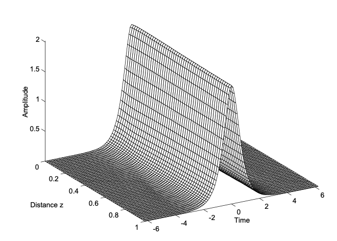
Figure 3.3 shows the numerical solution of the NSE for the fundamental soliton pulse. The distance, after which the soliton acquires a phase shift of \(\pi/4\), is called the soliton period, for reasons, which will become clear in the next section.

Since the dispersion is constant over the frequency, i.e. the NSE has no higher order dispersion, the center frequency of the soliton can be chosen arbitrarily. However, due to the dispersion, the group velocities of the solitons with different carrier frequencies will be different. One easily finds by a Gallilei transformation to a moving frame, that the NSE possess the following general fundamental soliton solution

\[A_s (z,t) = A_0 \text{sech} (x(z,t)) e^{-j \theta (z, t)}, \nonumber \]

with

\[x = \dfrac{1}{\tau} (t - 2|D_2|p_0 z - t_0), \nonumber \]

and a nonlinear phase shift

\[\theta = p_0 (t - t_0) + |D_2| \left (\dfrac{1}{\tau^2} - p_0^2 \right ) z + \theta_0. \nonumber \]

Thus, the energy fluence \(w\) or amplitude \(A_0\), the carrier frequency \(p_0\), the phase \(\theta_0\) and the origin \(t_0\), i.e. the timing of the fundamental soliton are not yet determined. Only the soliton area is fixed. The energy fluence and width are determined if one of them is specified, given a certain dispersion and SPM-coefficient.

Higher Order Solitons

The NSE has constant dispersion, in our case negative dispersion. That means the group velocity depends linearly on frequency. We assume, that two fundamental soltions are far apart from each other, so that they do not interact. Then this linear superpositon is for all practical purposes another solution of the NSE. If we choose the carrier frequency of the soliton, starting at a later time, higher than the one of the soliton in front, the later soliton will catch up with the leading soliton due to the negative dispersion and the pulses will collide.

Figure 3.4: A soliton with high carrier frequency collides with a soliton of lower carrier frequency. After the collison both pulses recover completely.

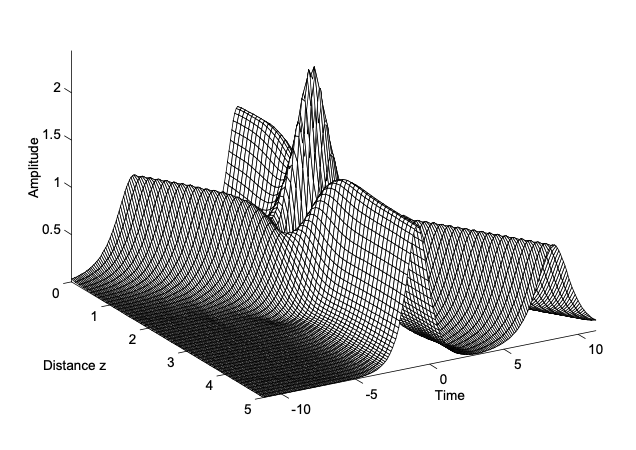
Figure 3.4 shows this situation. Obviously, the two pulses recover completely from the collision, i.e. the NSE has true soliton solutions. The solitons have particle like properties. A solution, composed of several fundamental solitons, is called a higher order soliton. If we look closer to figure 3.4, we recognize, that the soliton at rest in the local time frame, and which follows the \(t = 0\) line without the collision, is somewhat pushed forward due to the collision. A detailed analysis of the collision would also show, that the phases of the solitons have changed [4]. The phase changes due to soliton collisions are used to built all optical switches [10], using backfolded Mach-Zehnder interferometers, which can be realized in a self-stabilized way by Sagnac fiber loops.

Figure 3.5: (a) Amplitude and, (b) Spectrum of a higher order soliton composed of two fundamental solitons with the same carrier frequency

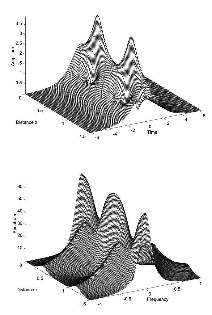
The NSE also shows higher order soliton solutions, that travel at the same speed, i.e. they posses the same carrier frequency, the so called breather solutions. Figures 3.5(a) and (b) show the amplitude and spectrum of such a higher order soliton solution, which has twice the area of the fundamental soliton. The simulation starts with a sech-pulse, that has twice the area of the fundamental soliton, shown in figure 3.3. Due to the interaction of the two solitons, the temporal shape and the spectrum exhibits a complicated but periodic behaviour. This period is the soliton period \(z = \pi/4\), as mentioned above. As can be seen from Figures 3.5(a) and 3.5(b), the higher order soliton dynamics leads to an enormous pulse shortening after half of the soliton period. This process has been used by Mollenauer, to build his soliton laser [11]. In the soliton laser, the pulse compression, that occures for a higher order soliton as shown in Figure 3.5(a), is exploited for modelocking. Mollenauer pioneered soliton propagation in optical fibers, as proposed by Hasegawa and Tappert [3], with the soliton laser, which produced the first picosecond pulses at 1.55 \(\mu\)m. A detailed account on the soliton laser is given by Haus [12].

So far, we have discussed the pure soliton solutions of the NSE. But, what happens if one starts propagation with an input pulse that does not correspond to a fundamental or higher order soliton?

Inverse Scattering Theory

Obviously, the NSE has solutions, which are composed of fundamental solitons. Thus, the solutions obey a certain superposition principle which is absolutely surprising for a nonlinear system. Of course, not arbitrary superpositions are possible as in a linear system. The deeper reason for the solution manyfold of the NSE can be found by studying its physical and mathematical properties. The mathematical basis for an analytic formulation of the solutions to the NSE is the inverse scattering theory [13, 14, 4, 15]. It is a spectral tranform method for solving integrable, nonlinear wave equations, similar to the Fourier transform for the solution of linear wave equations [16].

Figure 3.6: Fourier transform method for the solution of linear, time invariant partial differential equations.

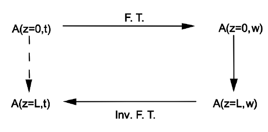
Let’s remember briefly, how to solve an initial value problem for a linear partial differential equation (p.d.e.), like Equation (2.6.12), that treats the case of a purely dispersive pulse propagation. The method is sketched in Figure 3.6. We Fourier tranform the initial pulse into the spectral domain, because, the exponential functions are eigensolutions of the differential operators with constant coefficients. The right side of (2.6.12) is only composed of powers of the differntial operator, therefore the exponentials are eigenfunctions of the complete right side. Thus, after Fourier transformation, the p.d.e. becomes a set of ordinary differential equations (o.d.e.), one for each partial wave. The excitation of each wave is given by the spectrum of the initial wave. The eigenvalues of the differential operator, that constitutes the right side of (2.6.12), is given by the dispersion relation, \(k(\omega)\), up to the imaginary unit. The solution of the remaining o.d.e is then a simple exponential of the dispersion relation. Now, we have the spectrum of the propagated wave and by inverse Fourier transformation, i.e. we sum over all partial waves, we find the new temporal shape of the propagated pulse.

As in the case of the Fourier transform method for the solution of linear wave equations, the inverse scattering theory is again based on a spectral transform, (Fig.3.7). However, this transform depends now on the details of the wave equation and the initial conditions. This dependence leads to a modified superposition principle. As is shown in [7], one can formulate for many integrable nonlinear wave equations a related scattering problem like one does in Quantum Theory for the scattering of a particle at a potential well. However, the potential well is now determined by the solution of the wave equation. Thus, the initial potential is already given by the initial conditions. The stationary states of the scattering problem, which are the eigensolutions of the corresponding Hamiltonian, are the analog to the monochromatic complex oscillations, which are the eigenfunctions of the differential operator. The eigenvalues are the analog to the dispersion relation, and as in the case of the linear p.d.e’s, the eigensolutions obey simple linear o.d.e’s.

Figure 3.7: Schematic representation of the inverse scattering theory for the solution of integrable nonlinear partial differential equations.

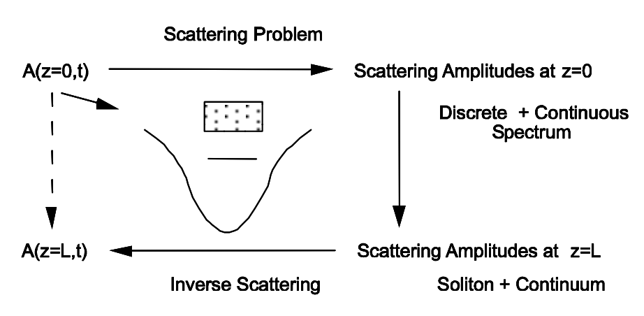
A given potential will have a certain number of bound states, that correspond to the discrete spectrum and a continuum of scattering states. The characteristic of the continuous eigenvalue spectrum is the reflection coefficient for waves scattered upon reflection at the potential. Thus, a certain potential, i.e. a certain initial condition, has a certain discrete spectrum and continuum with a corresponding reflection coefficient. From inverse scattering theory for quantum mechanical and electromagnetic scattering problems, we know, that the potential can be reconstructed from the scattering data, i.e. the reflection coefficient and the data for the discrete spectrum [?]. This is true for a very general class of scattering potentials. As one can almost guess now, the discrete eigenstates of the initial conditions will lead to soliton solutions. We have already studied the dynamics of some of these soliton solutions above. The continuous spectrum will lead to a dispersive wave which is called the continuum. Thus, the most general solution of the NSE, for given arbitrary initial conditions, is a superposition of a soliton, maybe a higher order soliton, and a continuum contribution.

The continuum will disperse during propagation, so that only the soliton is recognized after a while. Thus, the continuum becomes an asymptotically small contribution to the solution of the NSE. Therefore, the dynamics of the continuum is completely described by the linear dispersion relation of the wave equation.

The back transformation from the spectral to the time domain is not as simple as in the case of the Fourier transform for linear p.d.e’s. One has to solve a linear integral equation, the Marchenko equation [17]. Nevertheless, the solution of a nonlinear equation has been reduced to the solution of two linear problems, which is a tremendous success.

To appreciate these properties of the solutions of the NSE, we solve the NSE for a rectangular shaped initial pulse. The result is shown in Figure 3.8.

Figure 3.8: Solution of the NSE for an unchirped and rectangular shaped initial pulse.

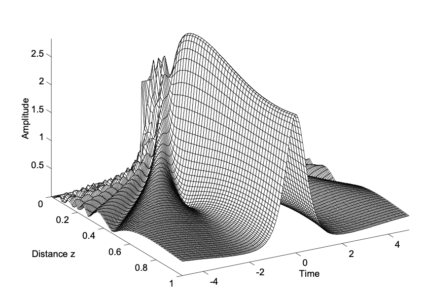
The scattering problem, that has to be solved for this initial condition, is the same as for a nonrelativistic particle in a rectangular potential box [32]. The depth of the potential is chosen small enough, so that it has only one bound state. Thus, we start with a wave composed of a fundamental soliton and continuum. It is easy to recognize the continuum contribution, i.e. the dispersive wave, that separates from the soliton during propagation. This solution illustrates, that soliton pulse shaping due to the presence of dispersion and self-phase modulation may have a strong impact on pulse generation [18]. When the dispersion and self-phase modulation are properly adjusted, soliton formation can lead to very clean, stable, and extremely short pulses in a mode-locked laser.