3.5: Soliton Perturbation Theory

From the previous discussion, we have full knowledge about the possible solutions of the NSE that describes a special Hamiltonian system. However, the NSE hardly describes a real physical system such as, for example, a real optical fiber in all its aspects [21, 22]. Indeed the NSE itself, as we have seen during the derivation in the previous sections, is only an approximation to the complete wave equation. We approximated the dispersion relation by a parabola at the assumed carrier frequency of the soliton. Also the instantaneous Kerr effect described by an intensity dependent refractive index is only an approximation to the real \(\chi^{(3)}\)-nonlinearity of a Kerr-medium [23, 24]. Therefore, it is most important to study what happens to a soliton solution of the NSE due to perturbing effects like higher order dispersion, finite response times of the nonlinearites, gain and the finite gain bandwidth of amplifiers, that compensate for the inevitable loss in a real system.

The investigation of solitons under perturbations is as old as the solitons itself. Many authors treat the perturbing effects in the scattering domain [25, 26]. Only recently, a perturbation theory on the basis of the linearized NSE has been developed, which is much more illustrative then a formulation in the scattering amplitudes. This was first used by Haus [27] and rigorously formulated by Kaup [28]. In this section, we will present this approach as far as it is indispensable for the following.

A system, where the most important physical processes are dispersion and self-phase modulation, is described by the NSE complimented with some perturbation term \(F\)

\[\dfrac{\partial A (z, t)}{\partial z} = -j \left [|D_2| \dfrac{\partial^2 A}{\partial t^2} + \delta |A|^2 A \right ] + F(A, A^*, z).\label{eq3.5.1} \]

In the following, we are interested what happens to a solution of the full equation (\(\ref{eq3.5.1}\)) which is very close to a fundamental soliton, i.e.

\[A(z, t) = \left [a\left(\dfrac{t}{\tau}\right) + \Delta A(z, t) \right ] e^{-jk_s z}.\label{eq3.5.2} \]

Here, \(a(x)\) is the fundamental soliton according to eq.(3.3.3)

\[a(\dfrac{t}{\tau}) = A_0 \text{sech} (\dfrac{t}{\tau}), \nonumber \]

and

\[k_s = \dfrac{1}{2} \delta A_0^2 \nonumber \]

is the phase shift of the soliton per unit length, i.e. the soltion wave vector.

A deviation from the ideal soliton can arise either due to the additional driving term \(F\) on the right side or due to a deviation already present in the initial condition. We use the form (\(\ref{eq3.5.2}\)) as an ansatz to solve the NSE to first order in the perturbation \(\Delta A\), i.e. we linearize the NSE around the fundamental soliton and obtain for the perturbation

\[\dfrac{\partial \Delta A}{\partial z} = -j k_s \left [\left(\dfrac{\partial^2}{\partial x^2} - 1\right) \Delta A + 2 \text{sech}^2(x) (2 \Delta A + \Delta A^*) \right ] + F(A, A^*, z) e^{jk_s z}, \label{eq3.5.5} \]

where \(x = t/\tau\). Due to the nonlinearity, the field is coupled to its complex conjugate. Thus, eq.(\(\ref{eq3.5.5}\)) corresponds actually to two equations, one for the amplitude and one for its complex conjugate. Therefore, we introduce the vector notation

\[\Delta A = \left (\begin{matrix} \Delta A \\ \Delta A^* \end{matrix} \right ). \nonumber \]

We further introduce the normalized propagation distance \(z' = k_s z\) and the normalized time \(x = t/\tau\). The linearized perturbed NSE is then given by

\[\dfrac{\partial}{\partial z'} \Delta A = L \Delta A + \dfrac{1}{k_s} F(A, A^*, z) e^{jz'}\label{eq3.5.7} \]

Here, \(\text{L}\) is the operator which arises from the linearization of the NSE

\[\text{L} = -j \sigma_3 \left [(\dfrac{\partial^2}{\partial x^2} - 1) + 2 \text{sech}^2 (x) (2 + \sigma_1) \right ],\label{eq3.5.8} \]

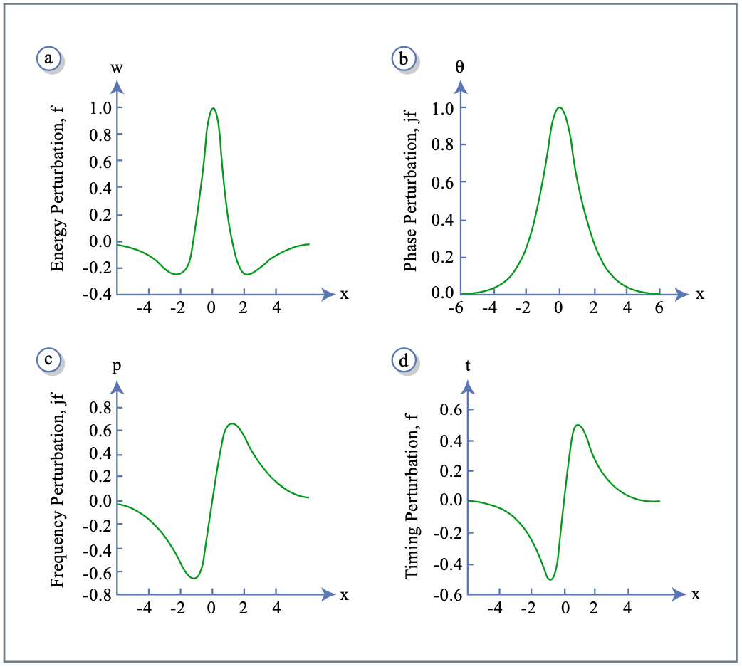
where \(\sigma_i, i = 1, 2, 3\) are the Pauli matrices. For a solution of the inhomogeneous equation (\(\ref{eq3.5.7}\)), we need the eigenfunctions and the spectrum of the differential operator \(\text{L}\). We found in section 3.3.2, that the fundamental soliton has four degrees of freedom, four free parameters. This gives already four known eigensolutions and mainsolutions of the linearized NSE, respectively. They are determined by the derivatives of the general fundamental soliton solutions according to Equations(3.3.9) to (3.3.11) with respect to free parameters. These eigenfunctions are

\[\text{f}_w (x) = \dfrac{1}{w} (1 - x \tanh x) a(x) \left (\begin{matrix} 1 \\ 1 \end{matrix} \right ), \nonumber \]

\[\text{f}_{\theta} (x) = -j a(x) \left (\begin{matrix} 1 \\ -1 \end{matrix} \right ), \nonumber \]

\[\text{f}_p (x) = -j x \tau a(x) \left (\begin{matrix} 1 \\ -1 \end{matrix} \right ), \nonumber \]

\[\text{f}_t (x) = \dfrac{1}{\tau} \tanh (x) a(x) \left (\begin{matrix} 1 \\ 1 \end{matrix} \right ), \nonumber \]

and they describe perturbations of the soliton energy, phase, carrier frequency and timing. One component of each of these vector functions is shown in Figure 3.9.

Figure 3.9: Perturabations in soliton amplitude (a), phase (b), frequency (c), and timing (d). Figure by MIT OCW.

The action of the evolution operator of the linearized NSE on these soliton perturbations is

\[\text{Lf}_w = \dfrac{1}{w} \text{f}_{\theta},\label{eq3.5.13} \]

\[\text{Lf}_{\theta} = 0, \nonumber \]

\[\text{Lf}_p = -2\tau^2 f_t,\label{eq3.5.15} \]

\[\text{Lf}_t = 0.\label{eq3.5.16} \]

Equations (\(\ref{eq3.5.13}\)) and (\(\ref{eq3.5.15}\)) indicate, that perturbations in energy and carrier frequency are converted to additional phase and timing fluctuations of the pulse due to SPM and GVD. This is the base for soliton squeezing in optical fibers [27]. The timing and phase perturbations can increase without bounds, because the system is autonomous, the origin for the Gordon-Haus effect, [29] and there is no phase reference in the system. The full continuous spectrum of the linearized NSE has been studied by Kaup [28] and is given by

\[\text{Lf}_k = \lambda_k \text{f}_k, \nonumber \]

\[\lambda_k = j (k^2+1), \nonumber \]

\[\text{f}_k(x) = e^{-jkx} \left (\begin{matrix} (k-j \tanh x)^2 \\ \text{sech}^2 x \end{matrix} \right ),\label{eq3.5.19} \]

and

\[\text{L}\bar{\text{f}}_k = \bar{\lambda}_k \bar{f}_k, \nonumber \]

\[\bar{\lambda}_k = -j (k^2 + 1), \nonumber \]

\[\bar{f}_k = \sigma_1 f_k.\label{eq3.5.22} \]

Our definition of the eigenfunctions is slightly different from Kaup [28], because we also define the inner product in the complex space as

\[< u|v > = \dfrac{1}{2} \int_{-\infty}^{+\infty} u^+ (x) v(x) dx.\label{eq3.5.23} \]

Adopting this definition, the inner product of a vector with itself in the subspace where the second component is the complex conjugate of the first component is the energy of the signal, a physical quantity.

The operator \(L\) is not self-adjoint with respect to this inner product. The physical origin for this mathematical property is, that the linearized system does not conserve energy due to the parametric pumping by the soliton. However, from (\(\ref{eq3.5.8}\)) and (\(\ref{eq3.5.23}\)), we can easily see that the adjoint operator is given by

\[\text{L}^{+} = -\sigma_3 \text{L} \sigma_3, \nonumber \]

and therefore, we obtain for the spectrum of the adjoint operator

\[\text{L}^{+} \text{f}_k^{(+)} = \lambda_{k}^{(+)} \text{f}_k^{(+)},\label{eq3.5.25} \]

\[\lambda_{k}^{(+)} = -j (k^2 + 1), \nonumber \]

\[\text{f}_k^{(+)} = \dfrac{1}{\pi (k^2 + 1)^2} \sigma_3 \text{f}_k, \nonumber \]

and

\[\text{L}^{+} \bar{\text{f}}_k^{(+)} = \bar{\lambda}_{k}^{(+)} \bar{\text{f}}_k^{(+)}, \nonumber \]

\[\bar{\lambda}_{k}^{(+)} = j (k^2 + 1), \nonumber \]

\[\bar{\text{f}}_k^{(+)} = \dfrac{1}{\pi (k^2 + 1)^2} \sigma_3 \bar{\text{f}}_k, \nonumber \]

The eigenfunctions to \(\text{L}\) and its adjoint are mutually orthogonal to each other, and they are already properly normalized

\[<\text{f}_k^{(+)}|\text{f}_{k'} > = \delta (k - k')\nonumber \]

\[<\bar{\text{f}}_k^{(+)}|\bar{\text{f}}_{k'} > = \delta (k - k')\nonumber \]

\[<\bar{\text{f}}_k^{(+)}|\text{f}_{k'} > = <\text{f}_k^{(+)} |\bar{\text{k}}_{k'} >=0.\nonumber \]

This system, which describes the continuum excitations, is made complete by taking also into account the perturbations of the four degrees of freedom of the soliton (\(\ref{eq3.5.13}\)) - (\(\ref{eq3.5.16}\)) and their adjoints

\[\text{f}_w^{(+)} (x) = j 2 \tau \sigma_3 \text{f}_{\theta} (x) = 2 \tau a(x) \left ( \begin{matrix} 1 \\ 1 \end{matrix} \right ),\label{eq3.5.31} \]

\[\begin{array} {rcl} {\text{f}_{\theta}^{(+)} (x)} & = & {-2j \tau \sigma_3 \text{f}_w (x)} \\ {} & = & {\dfrac{-2j\tau}{w} (1 - x \tanh x) a(x) \left ( \begin{matrix} 1 \\ -1 \end{matrix} \right ),}\end{array} \nonumber \]

\[\text{f}_p^{(+)} (x) = -\dfrac{2j\tau}{w} \sigma_3 \text{f}_t (x) = \dfrac{2i}{w} \tanh a(x) \left ( \begin{matrix} 1 \\ -1 \end{matrix} \right ), \nonumber \]

\[\text{f}_t^{(+)} (x) = \dfrac{2j\tau}{w} \sigma_3 \text{f}_p (x) = \dfrac{2 \tau^2}{w} xa(x) \left ( \begin{matrix} 1 \\ 1 \end{matrix} \right ). \nonumber \]

Now, the unity can be decomposed into two projections, one onto the continuum and one onto the perturbation of the soliton variables [28]

\[\begin{array} {rcl} {\delta (x - x')} & = & {\int_{-\infty}^{\infty} dk [|\text{f}_k >< \text{f}_k^{(+)}| + |\bar{\text{f}}_{k} >< \bar{\text{f}}_{k}^{(+)}|]} \\ {} & + & {|\text{f}_w >< \text{f}_w^{(+)}| + |\text{f}_{\theta} >< \text{f}_{\theta}^{(+)}|} \\ {} & + & {|\text{f}_p >< \text{f}_p^{(+)}| + |\text{f}_t >< \text{f}_t^{(+)}|}. \end{array} \nonumber \]

Any deviation \(\Delta A\) can be decomposed into a contribution that leads to a soliton with a shift in the four soliton paramters and a continuum contribution \(a_c\)

\[\Delta A (z') = \Delta w (z') \text{f}_w + \Delta \theta (z') \text{f}_{\theta} + \Delta p(z') \text{f}_p + \Delta t(z') \text{f}_t + \text{a}_c (z').\label{eq3.5.36} \]

Further, the continuum can be written as

\[\text{a}_c = \int_{-\infty}^{\infty} dk [g(k) \text{f}_k (x) + \bar{g} (k) \bar{\text{f}}_k (x)].\label{eq3.5.37} \]

If we put the decomposition (\(\ref{eq3.5.36}\)) into (\(\ref{eq3.5.7}\)) we obtain

\[\dfrac{\partial \Delta w}{\partial z'} \text{f}_w + \dfrac{\partial \Delta \theta}{\partial z'} \text{f}_{\theta} + \dfrac{\partial \Delta p}{\partial z'} \text{f}_p + \dfrac{\partial \Delta t}{\partial z'} \text{f}_t + \dfrac{\partial}{\partial z'} \text{a}_c = \nonumber \]

\[\text{L} (\Delta w(z') \text{f}_w + \Delta p (z') \text{f}_p + \text{a} (z')_c) + \dfrac{1}{k_s} \text{F} (A, A^*, z') e^{-iz'}. \nonumber \]

By building the scalar products (\(\ref{eq3.5.23}\)) of this equation with the eigensolutions of the adjoint evolution operator (\(\ref{eq3.5.25}\)) to (\(\ref{eq3.5.31}\)) and using the eigenvalues (\(\ref{eq3.5.13}\)) to (\(\ref{eq3.5.22}\)), we find

\[\dfrac{\partial}{\partial z'} \Delta w = \dfrac{1}{k_s} < \text{f}_w^{(+)} | \text{F} e^{jz'} >, \nonumber \]

\[\dfrac{\partial}{\partial z'} \Delta \theta = \dfrac{\Delta W}{W} + \dfrac{1}{k_s} < \text{f}_{\theta}^{(+)} | \text{F} e^{jz'} >, \nonumber \]

\[\dfrac{\partial}{\partial z'} \Delta p = \dfrac{1}{k_s} < \text{f}_p^{(+)} | \text{F} e^{jz'} >, \nonumber \]

\[\dfrac{\partial}{\partial z'} \Delta t = 2 \tau \Delta p + \dfrac{1}{k_s} < \text{f}_t^{(+)} | \text{F} e^{jz'} >, \nonumber \]

\[\dfrac{\partial}{\partial z'} g(k) = j(1 + k^2) g(k) + \dfrac{1}{k_s} < \text{f}_k^{(+)} \text{F}(A, A^*, z') e^{jz'} >.\label{3.5.43} \]

Note, that the continuum \(\text{a}_c\) has to be in the subspace defined by

\[\sigma_1 \text{a}_c = \text{a}_c^*.\label{eq3.5.44} \]

The spectra of the continuum \(g(k)\) and \(\bar{g}(k)\) are related by

\[\bar{g} (k) = g(-k)^*. \nonumber \]

Then, we can directly compute the continuum from its spectrum using (\(\ref{eq3.5.19}\)), (\(\ref{eq3.5.37}\)) and (\(\ref{eq3.5.44}\))

\[a_c = -\dfrac{\partial^2 G(x)}{\partial x^2} + 2 \tanh (x) \dfrac{\partial G(x)}{\partial x} - \tanh^2 (x) G(x) + G^* (x) \text{sech}^2 (x),\label{eq3.5.46} \]

where \(G(x)\) is, up to the phase factor \(e^{iz'}\), Gordon’s associated function [33]. It is the inverse Fourier transform of the spectrum

\[G(x) = \int_{-\infty}^{\infty} g(k) e^{ikx} dk.\label{eq3.5.47} \]

Since \(g(k)\) obeys eq.(\(\ref{eq3.5.44}\)), Gordon’s associated function obeys a pure dispersive equation in the absence of a driving term \(F\)

\[\dfrac{\partial G(z', x)}{\partial z'} = -j \left ( 1 + \dfrac{\partial ^2}{\partial x^2} \right ) G(z', x). \nonumber \]

It is instructive to look at the spectrum of the continuum when only one continuum mode with normalized frequency \(k_0\) is present, i.e. \(g(k) = \delta (k - k_0)\). Then according to Equations (\(\ref{eq3.5.46}\)) and (\(\ref{eq3.5.47}\)) we have

\[a_{c,k} (x) = [k_0^2 - 2j k_0 \tanh (x) - 1] e^{-jk_0x} + 2 \text{sech}^2 (x) \cos (x). \nonumber \]

The spectrum of this continuum contribution is

\[\begin{array} {rcl} {\bar{a}_{c, k} (\omega)} & = & {2\pi (k_)^2 - 1) \delta (\omega - k_0) +2k_0 P.V. \left (\dfrac{2}{\omega - k_0} + \dfrac{\pi}{\sinh(\tfrac{\pi}{2} (\omega - k_0))} \right )} \\ {} & = & {+\pi \dfrac{\omega - k_0}{\sinh (\tfrac{\pi}{2} (\omega - k_0))} + \pi \dfrac{\omega + k_0}{\sinh (\tfrac{\pi}{2} (\omega + k_0))}}\end{array} \nonumber \]