3.6: Soliton Instabilities by Periodic Perturbations

Periodic perturbations of solitons are important for understanding ultrashort pulse lasers as well as long distance optical communication systems [30, 31]. Along a long distance transmission system, the pulses have to be periodically amplified. In a mode-locked laser system, most often the nonlinearity, dispersion and gain occur in a lumped manner. The solitons propagating in these systems are only average solitons, which propagate through discrete components in a periodic fashion, as we will see later.

The effect of this periodic perturbations can be modeled by an additional term \(F\) in the perturbed NSE according to Equation (3.5.1)

\[F(A, A^*, z) = j \xi \sum_{n = -\infty}^{\infty} \delta (z - nz_A) A(z,t). \nonumber \]

The periodic kicking of the soliton leads to shedding of energy into continuum modes according to Equation (3.5.43)

\[\dfrac{\partial}{\partial z} g(k) = jk_s (1 + k^2)g(k) + \langle \text{f}_k^{(+)} \text{F} (A, A^*, z) e^{jk_s z} \rangle. \nonumber \]

\[\begin{align*} \langle \text{f}_{k}^{(+)} \text{F} (A, A^*, z) e^{jk_s z} \rangle &= j \xi \sum_{n = -\infty}^{\infty} \delta (z - nz_A) \dfrac{1}{2} \cdot \int_{-\infty}^{+\infty} \dfrac{1}{\pi (k^2 + 1)^2} e^{jkx} \left (\begin{matrix} (k + j \tanh x)^2 \\ -\text{sech}^2 x \end{matrix} \right ) \cdot \left ( \begin{matrix} 1 \\ 1 \end{matrix} \right ) A_0 \text{sech} x\ dx\\[4pt] &=j \xi \sum_{n = -\infty}^{\infty} \delta (z - n z_A) \cdot \int_{-\infty}^{+\infty} \dfrac{A_0}{2\pi (k^2 + 1)^2} e^{jkx} (k^2 + 2jk \tanh x - 1) \cdot \text{sech} x\ dx \end{align*} \nonumber \]

Note, \(\tfrac{d}{dx} \text{sech} x = -\text{sech} x \tanh x\), and therefore

\[\begin{align*} \langle \text{f}_k^{(+)} \text{F} (A, A^*, z) e^{jz} \rangle &= -j \xi \sum_{n = -\infty}^{\infty} \delta (z - nz_A) \cdot \int_{-\infty}^{+\infty} \dfrac{A_0}{2\pi (k^2 + 1)} e^{jkx} \cdot \text{sech} x dx \\&= -j \xi \sum_{n = -\infty}^{\infty} \delta (z - nz_A) \dfrac{A_0}{4(k^2 + 1)} \text{sech} (\dfrac{\pi k}{2}). \end{align*} \nonumber \]

Using \(\sum_{n = -\infty}^{\infty} \delta (z - nz_A) = \dfrac{1}{z_A} \sum_{m = -\infty}^{\infty} e^{jm \tfrac{2\pi}{z_A} z}\) we obtain

\[\dfrac{\partial}{\partial z} g(k) = jk_s (1 + k^2) g(k) - j \dfrac{\xi}{z_A} \sum_{m =-\infty}^{\infty} e^{jm \tfrac{2\pi}{z_A} z} \dfrac{A_0}{4(k^2 + 1)} \text{sech} \left(\dfrac{\pi k}{2}\right).\label{eq3.6.6} \]

Equation \ref{eq3.6.6} is a linear differential equation with constant coefficients for the continuum amplitudes \(g(k)\), which can be solved by variation of constants with the ansatz

\[g(k,z) = C(k, z) e^{jk_s (1 + k^2) z}, \nonumber \]

and initial conditions \(C(z = 0) = 0\), we obtain

\[\dfrac{\partial}{\partial z} C(k, z) = -j \dfrac{\xi}{z_A} \sum_{m = -\infty}^{\infty} \dfrac{A_0}{4(k^2+1)} \text{sech} \left(\dfrac{\pi k}{2}\right) e^{-j(k_s (1 + k^2) - m \tfrac{2\pi}{z_A} z)}, \nonumber \]

or

\[\begin{align*} C(k,z) &= -j \dfrac{\xi}{z_A} \dfrac{A_0}{4(k^2+1)} \text{sech} \left(\dfrac{\pi k}{2} \right) \cdot \sum_{m = -\infty}^{\infty} \int_0^z e^{j(-k_s (1 + k^2) + m \tfrac{2\pi}{z_A})z} dz \\[4pt] &= -j\dfrac{\xi}{z_A} \dfrac{A_0}{4(k^2+1)} \text{sech} \left(\dfrac{\pi k}{2}\right) \cdot \sum_{m = -\infty}^{\infty} \dfrac{e^{j(-k_s (1 + k^2) + m \tfrac{2\pi}{z_A})z} - 1}{m\tfrac{2\pi}{z_A} - k_s (1 + k^2)}. \end{align*} \nonumber \]

There is a resonant denominator, which blows up at certain normalized frequencies \(k_m\) for \(z \to \infty\) Those frequencies are given by

\[m \dfrac{2\pi}{z_A} - k_s (1 + k_m^2) = 0 \nonumber \]

or

\[ k_m = \pm \sqrt{\dfrac{m\tfrac{2\pi}{z_A}}{k_s} - 1}. \nonumber \]

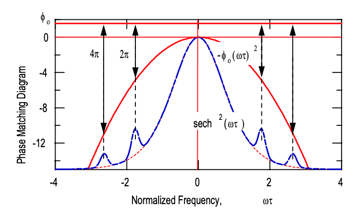
Removing the normalization by setting \(k = \omega \tau\), \(k_s =|D_2|/\tau^2\) and introducing the nonlinear phase shift of the soliton acquired over one period of the perturbation \(\phi_0 = k_s z_A\), we obtain a handy formula for the location of the resonant sidebands

\[\omega_m = \pm \dfrac{1}{\tau} \sqrt{\dfrac{2m \pi}{\phi_0} - 1}, \nonumber \]

and the coefficients

\[C(\omega, z) = -j \dfrac{\xi}{z_A} \dfrac{A_0}{4((\omega \tau)^2 + 1)} \text{sech} (\dfrac{\pi \omega \tau}{2}) \cdot \sum_{m = -\infty}^{\infty} z_A \dfrac{e^{j(-k_s (1 + (\omega \tau)^2) + m \tfrac{2\pi}{z_A})z} - 1}{2 \pi m - \phi_0 (1 + (\omega \tau)^2)}. \nonumber \]

The coefficients stay bounded for frequencies not equal to the resonant condition and they grow linearly with \(z_A\), at resonance, which leads to a destruction of the pulse. To stabilize the soliton against this growth of resonant sidebands, the resonant frequencies have to stay outside the spectrum of the soliton, see Figure 3.10, which feeds the continuum, i.e. \(\omega_m \gg \tfrac{1}{\tau}\). This condition is only fulfilled if \(\phi_0 \ll \dfrac{\pi}{4}\). This condition requires that the soliton period is much longer than the period of the perturbation. As an example Figure 3.10 shows the resonant sidebands observed in a fiber laser. For optical communication systems this condition requires that the soliton energy has to be kept small enough, so that the soliton period is much longer than the distance between amplifiers, which constitute periodic perturbations to the soliton. These sidebands are often called Kelly sidebands, according to the person who first described its origin properly [30].

Figure 3.10: Phasematching between soliton and continuum due to periodic perturbations leads to resonant sideband generation. The case shown is for \(\phi_0 = \pi/2\).

To illustrate its importance we discuss the spectrum observed from the long cavity Ti:sapphire laser system illustrated in Figure 3.11 and described in full detail in [37]. Due to the low repetition rate, a rather large pulse energy builds up in the cavity, which leads to a large nonlinear phase shift per roundtrip.

Figure 3.11: Schematic layout of a high pulse energy laser cavity. All shaded mirrors are (Double-chirped mirrors) DCMs. The standard 100 MHz cavity with arms of 45 cm and 95 cm extends from the OC to M6 for the short and long arms respectively. The multiple pass cavity (MPC) is enclosed in the dotted box. The pump source is a frequency doubled Nd:Vanadate that produces up to 10 W at 532 nm [37]. Kowalewicz, A. M., et al. "Generation of 150-nJ pulses from a multiple-pass cavity Kerr-lens modelocked \(\ce{Ti:Al2O3}\) oscillator." Optics Letters 28 (2003): 1507-09.

Figure 3.12 shows the spectrum of the output from the laser. The Kelly sidebands are clearly visible. It is this kind of instability, which limits further increase in pulse energy from these systems operating in the soliton pulse shaping regime. Energy is drained from the main pulse into the sidebands, which grow at the expense of the pulse. At some point the pulse shaping becomes unstable because of conditions to be discussed in later chapters.

Figure 3.12: Measured modelocked spectrum with a 16.5 nm FWHM centered at 788 nm. Kowalewicz, A. M., et al. "Generation of 150-nJ pulses from a multiple-pass cavity Kerr-lens modelocked \(\ce{Ti:Al2O3}\) oscillator." Optics Letters 28 (2003): 1507-09.