4.4: Q-Switching
- Page ID
- 44654
\( \newcommand{\vecs}[1]{\overset { \scriptstyle \rightharpoonup} {\mathbf{#1}} } \)
\( \newcommand{\vecd}[1]{\overset{-\!-\!\rightharpoonup}{\vphantom{a}\smash {#1}}} \)
\( \newcommand{\dsum}{\displaystyle\sum\limits} \)
\( \newcommand{\dint}{\displaystyle\int\limits} \)
\( \newcommand{\dlim}{\displaystyle\lim\limits} \)
\( \newcommand{\id}{\mathrm{id}}\) \( \newcommand{\Span}{\mathrm{span}}\)
( \newcommand{\kernel}{\mathrm{null}\,}\) \( \newcommand{\range}{\mathrm{range}\,}\)
\( \newcommand{\RealPart}{\mathrm{Re}}\) \( \newcommand{\ImaginaryPart}{\mathrm{Im}}\)
\( \newcommand{\Argument}{\mathrm{Arg}}\) \( \newcommand{\norm}[1]{\| #1 \|}\)
\( \newcommand{\inner}[2]{\langle #1, #2 \rangle}\)
\( \newcommand{\Span}{\mathrm{span}}\)
\( \newcommand{\id}{\mathrm{id}}\)
\( \newcommand{\Span}{\mathrm{span}}\)
\( \newcommand{\kernel}{\mathrm{null}\,}\)
\( \newcommand{\range}{\mathrm{range}\,}\)
\( \newcommand{\RealPart}{\mathrm{Re}}\)
\( \newcommand{\ImaginaryPart}{\mathrm{Im}}\)
\( \newcommand{\Argument}{\mathrm{Arg}}\)
\( \newcommand{\norm}[1]{\| #1 \|}\)
\( \newcommand{\inner}[2]{\langle #1, #2 \rangle}\)
\( \newcommand{\Span}{\mathrm{span}}\) \( \newcommand{\AA}{\unicode[.8,0]{x212B}}\)
\( \newcommand{\vectorA}[1]{\vec{#1}} % arrow\)
\( \newcommand{\vectorAt}[1]{\vec{\text{#1}}} % arrow\)
\( \newcommand{\vectorB}[1]{\overset { \scriptstyle \rightharpoonup} {\mathbf{#1}} } \)
\( \newcommand{\vectorC}[1]{\textbf{#1}} \)
\( \newcommand{\vectorD}[1]{\overrightarrow{#1}} \)
\( \newcommand{\vectorDt}[1]{\overrightarrow{\text{#1}}} \)
\( \newcommand{\vectE}[1]{\overset{-\!-\!\rightharpoonup}{\vphantom{a}\smash{\mathbf {#1}}}} \)
\( \newcommand{\vecs}[1]{\overset { \scriptstyle \rightharpoonup} {\mathbf{#1}} } \)
\( \newcommand{\vecd}[1]{\overset{-\!-\!\rightharpoonup}{\vphantom{a}\smash {#1}}} \)
\(\newcommand{\avec}{\mathbf a}\) \(\newcommand{\bvec}{\mathbf b}\) \(\newcommand{\cvec}{\mathbf c}\) \(\newcommand{\dvec}{\mathbf d}\) \(\newcommand{\dtil}{\widetilde{\mathbf d}}\) \(\newcommand{\evec}{\mathbf e}\) \(\newcommand{\fvec}{\mathbf f}\) \(\newcommand{\nvec}{\mathbf n}\) \(\newcommand{\pvec}{\mathbf p}\) \(\newcommand{\qvec}{\mathbf q}\) \(\newcommand{\svec}{\mathbf s}\) \(\newcommand{\tvec}{\mathbf t}\) \(\newcommand{\uvec}{\mathbf u}\) \(\newcommand{\vvec}{\mathbf v}\) \(\newcommand{\wvec}{\mathbf w}\) \(\newcommand{\xvec}{\mathbf x}\) \(\newcommand{\yvec}{\mathbf y}\) \(\newcommand{\zvec}{\mathbf z}\) \(\newcommand{\rvec}{\mathbf r}\) \(\newcommand{\mvec}{\mathbf m}\) \(\newcommand{\zerovec}{\mathbf 0}\) \(\newcommand{\onevec}{\mathbf 1}\) \(\newcommand{\real}{\mathbb R}\) \(\newcommand{\twovec}[2]{\left[\begin{array}{r}#1 \\ #2 \end{array}\right]}\) \(\newcommand{\ctwovec}[2]{\left[\begin{array}{c}#1 \\ #2 \end{array}\right]}\) \(\newcommand{\threevec}[3]{\left[\begin{array}{r}#1 \\ #2 \\ #3 \end{array}\right]}\) \(\newcommand{\cthreevec}[3]{\left[\begin{array}{c}#1 \\ #2 \\ #3 \end{array}\right]}\) \(\newcommand{\fourvec}[4]{\left[\begin{array}{r}#1 \\ #2 \\ #3 \\ #4 \end{array}\right]}\) \(\newcommand{\cfourvec}[4]{\left[\begin{array}{c}#1 \\ #2 \\ #3 \\ #4 \end{array}\right]}\) \(\newcommand{\fivevec}[5]{\left[\begin{array}{r}#1 \\ #2 \\ #3 \\ #4 \\ #5 \\ \end{array}\right]}\) \(\newcommand{\cfivevec}[5]{\left[\begin{array}{c}#1 \\ #2 \\ #3 \\ #4 \\ #5 \\ \end{array}\right]}\) \(\newcommand{\mattwo}[4]{\left[\begin{array}{rr}#1 \amp #2 \\ #3 \amp #4 \\ \end{array}\right]}\) \(\newcommand{\laspan}[1]{\text{Span}\{#1\}}\) \(\newcommand{\bcal}{\cal B}\) \(\newcommand{\ccal}{\cal C}\) \(\newcommand{\scal}{\cal S}\) \(\newcommand{\wcal}{\cal W}\) \(\newcommand{\ecal}{\cal E}\) \(\newcommand{\coords}[2]{\left\{#1\right\}_{#2}}\) \(\newcommand{\gray}[1]{\color{gray}{#1}}\) \(\newcommand{\lgray}[1]{\color{lightgray}{#1}}\) \(\newcommand{\rank}{\operatorname{rank}}\) \(\newcommand{\row}{\text{Row}}\) \(\newcommand{\col}{\text{Col}}\) \(\renewcommand{\row}{\text{Row}}\) \(\newcommand{\nul}{\text{Nul}}\) \(\newcommand{\var}{\text{Var}}\) \(\newcommand{\corr}{\text{corr}}\) \(\newcommand{\len}[1]{\left|#1\right|}\) \(\newcommand{\bbar}{\overline{\bvec}}\) \(\newcommand{\bhat}{\widehat{\bvec}}\) \(\newcommand{\bperp}{\bvec^\perp}\) \(\newcommand{\xhat}{\widehat{\xvec}}\) \(\newcommand{\vhat}{\widehat{\vvec}}\) \(\newcommand{\uhat}{\widehat{\uvec}}\) \(\newcommand{\what}{\widehat{\wvec}}\) \(\newcommand{\Sighat}{\widehat{\Sigma}}\) \(\newcommand{\lt}{<}\) \(\newcommand{\gt}{>}\) \(\newcommand{\amp}{&}\) \(\definecolor{fillinmathshade}{gray}{0.9}\)Image removed due to copyright restrictions. Please see: Keller, U., Ultrafast Laser Physics, Institute of Quantum Electronics, Swiss Federal Institute of Technology, ETH Hönggerberg—HPT, CH-8093 Zurich, Switzerland.
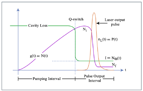
Figure 4.5: Gain and loss dynamics of an actively Q-switched laser.
The energy stored in the laser medium can be released suddenly by increasing the Q-value of the cavity so that the laser reaches threshold. This can be done actively, for example by quickly moving one of the resonator mirrors in place or passively by placing a saturable absorber in the resonator [1, 16]. Hellwarth was first to suggest this method only one year after the invention of the laser. As a rough orientation for a solid-state laser, the following relation for the relevant time scales is generally valid
\[\tau_L \gg T_R \gg \tau_p. \nonumber \]
Active Q-Switching
Figure 4.5 shows the principle dynamics of an actively Q-switched laser. The laser is pumped by a pump pulse with a length on the order of the upper- state lifetime, while the intracavity losses are kept high enough, so that the laser can not reach threshold. Therefore, the laser medium acts as an energy storage. The energy only relaxes by spontenous and nonradiative transitions. Then suddenly the intracavity loss is reduced, for example by a rotating cavity mirror. The laser is pumped way above threshold and the light field builts up exponentially with the net gain until the pulse energy comes close to the saturation energy of the gain medium. The gain saturates and is extracted, so that the laser is shut off by the pulse itself.
A typical actively Q-switched pulse is asymmetric: The rise time is pro- portional to the net gain after the Q-value of the cavity is actively switched to a high value. The light intensity growths proportional to \(2g_0/T_R\). When the gain is depleted, the fall time mostly depends on the cavity decay time τp. For short Q-switched pulses a short cavity length, high gain and a large change in the cavity Q is necessary. If the Q-switch is not fast, the pulse width may be limited by the speed of the switch. Typical electro-optical and acousto-optical switches are 10 ns and 50 ns, respectively
Image removed due to copyright restrictions. Please see: Keller, U., Ultrafast Laser Physics, Institute of Quantum Electronics, Swiss Federal Institute of Technology, ETH Hönggerberg—HPT, CH-8093 Zurich, Switzerland.
Figure 4.6: Asymmetric actively Q-switched pulse.
For example, with a diode-pumped \(\ce{Nd:YAG}\) microchip laser [6] using an electro-optical switch based on \(\ce{LiTaO3}\) Q-switched pulses as short as 270 ps at repetition rates of 5 kHz, peak powers of 25 kW at an average power of 34 mW, and pulse energy of 6.8 \(\mu\)J have been generated (Figure 4.7).
Image removed due to copyright restrictions. Please see: Kafka, J. D., and T. Baer. "Mode-locked erbium-doped fiber laser with soliton pulse shaping." Optics Letters 14 (1989): 1269-1271.
Figure 4.7: Q-switched microchip laser using an electro-optic switch. The pulse is measured with a sampling scope [8]
Similar results were achieved with Nd:YLF [7] and the corresponding setup is shown in Figure 4.8.
Single-Frequency Q-Switched Pulses
Q-switched lasers only deliver stable output if they oscillate single frequency. Usually this is not automatically achieved. One method to achieve this is by seeding with a single-frequency laser during Q-switched operation, so that there is already a population in one of the longitudinal modes before the pulse is building up. This mode will extract all the energy before the other modes can do, see Figure 4.9
Image removed due to copyright restrictions. Please see: Keller, U., Ultrafast Laser Physics, Institute of Quantum Electronics, Swiss Federal Institute of Technology, ETH Hönggerberg—HPT, CH-8093 Zurich, Switzerland.
Figure 4.9: Output intenisity of a Q-switched laser without a) and with seeding b).
Another possibility to achieve single-mode output is either using an etalon in the cavity or making the cavity so short, that only one longitudinal mode is within the gain bandwidth (Figure 4.10). This is usually only the case if the cavity length is on the order of a view millimeters or below.The microchip laser [6][11][10] can be combined with an electro-optic modulator to achieve very compact high peak power lasers with subnanosecond pulsewidth (Figure 4.7).
Image removed due to copyright restrictions. Please see: Keller, U., Ultrafast Laser Physics, Institute of Quantum Electronics, Swiss Federal Institute of Technology, ETH Hönggerberg—HPT, CH-8093 Zurich, Switzerland.
Figure 4.10: In a microchip laser the resonator can be so short, that there is only one longitudinal mode within the gain bandwidth.
Theory of Active Q-Switching
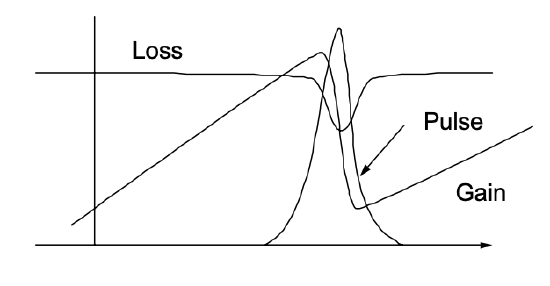
We want to get some insight into the pulse built-up and decay of the actively Q-switched pulse. We consider the ideal situation, where the loss of the laser cavity can be instantaneously switched from a high value to a low value, i.e. the quality factor is switched from a low value to a high value, respectively (Figure: 4.11)
Pumping Interval
During pumping with a constant pump rate \(R_p\), proportional to the small signal gain \(\text{g}_0\), the inversion is built up. Since there is no field present, the gain follows the simple equation:
\[\dfrac{d}{dt} \text{g} = -\dfrac{\text{g} - \text{g}_0}{\tau_L}, \nonumber \]
or
\[\text{g}(t) = \text{g}_0 (1 - e^{-t/\tau_L}), \nonumber \]
Pulse Built-up-Phase:
Assuming an instantaneous switching of the cavity losses we look for an approximate solution to the rate equations starting of with the initial gain or inversion \(\text{g}_i = hf_LN_{2i}/(2E_{sat}) = hf_LN_i/(2E_{sat})\), we can savely leave the index away since there is only an upper state population. We further assume that during pulse built-up the stimulated emission rate is the dominate term changing the inversion. Then the rate equations simplify to \(\tau\)
\[\dfrac{d}{dt} \text{g} = -\dfrac{\text{g}P}{E_{sat_p}} \nonumber \]
\[\dfrac{d}{dt} P = \dfrac{2(\text{g} - l)}{T_R} P, \nonumber \]
resulting in
\[\dfrac{dP}{d\text{g}} = \dfrac{2E_{sat}}{T_R} \left (\dfrac{l}{\text{g}} - 1\right ).\label{eq4.4.6} \]
We use the following inital conditions for the intracavity power \(P (t = 0) = 0\) and initial gain \(\text{g}(t = 0) = \text{g}_i = r \cdot l\). Note, \(r\) means how many times the laser is pumped above threshold after the Q-switch is operated and the intracavity losses have been reduced to \(l\). Then \(\ref{eq4.4.6}\) can be directly solved and we obtain
\[P(t) = \dfrac{2 E_{sat}}{T_R} \left (\text{g}_i - \text{g} (t) + l \ln \dfrac{\text{g} (t)}{\text{g}_i} \right ). \nonumber \]
From this equation we can deduce the maximum power of the pulse, since the growth of the intracavity power will stop when the gain is reduced to the losses, \(g(t) = l\), (Figure 4.11)
\[P_{\max} = \dfrac{2lE_{sat}}{T_R} (r - 1 - \ln r) \nonumber \]
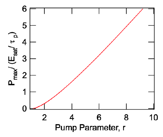
\[= \dfrac{E_{sat}}{\tau_p} (r - 1 - \ln r).\label{eq4.4.9} \]
This is the first important quantity of the generated pulse and is shown normalized in Figure 4.12.
Next, we can find the final gain \(\text{g}_f\), that is reached once the pulse emission is completed, i.e. that is when the right side of (4.38) vanishes
\[\left (\text{g}_i - \text{g}_f + l \ln \left ( \dfrac{\text{g}_f}{\text{g}_i} \right ) \right ) = 0 \nonumber \]
Using the pump parameter \(r = \text{g}_i/l\), this gives as an expression for the ratio between final and initial gain or between final and initial inversion
\[1 - \dfrac{\text{g}_f}{\text{g}_i} + \dfrac{1}{r} \ln \left (\dfrac{\text{g}_f}{\text{g}_i} \right ) = 0, \nonumber \]
\[1 - \dfrac{N_f}{N_i} + \dfrac{1}{r} \ln \left ( \dfrac{N_f}{N_i} \right ) = 0,\label{eq4.4.12} \]
which depends only on the pump parameter. Assuming further, that there are no internal losses, then we can estimate the pulse energy generated by
\[E_P = (N_i - N_f) h f_L. \nonumber \]
This is also equal to the output coupled pulse energy since no internal losses are assumed. Thus, if the final inversion gets small all the energy stored in the gain medium can be extracted. We define the energy extraction efficiency \(\eta\)
\[\eta = \dfrac{N_i - N_f}{N_i}, \nonumber \]
that tells us how much of the initially stored energy can be extracted using eq.(\(\ref{eq4.4.12}\))
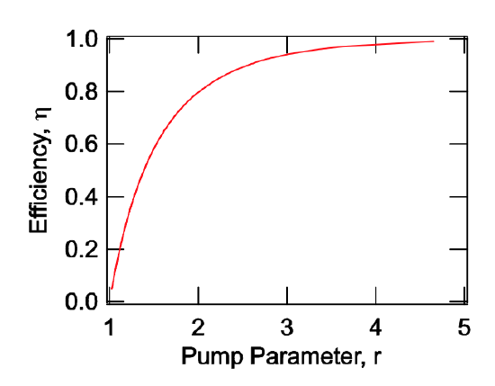
\[\eta + \dfrac{1}{r} \ln (1 - \eta) = 0. \nonumber \]
This efficiency is plotted in Figure 4.13.
Note, the energy extraction efficiency only depends on the pump parameter \(r\). Now, the emitted pulse energy can be written as
\[E_P = \eta (r) N_i h f_L.\label{eq4.4.16} \]
and we can estimate the pulse width of the emitted pulse by the ratio between pulse energy and peak power using (\(\ref{eq4.4.9}\)) and (\(\ref{eq4.4.16}\))
\[\begin{array} {rcl} {\tau_{Pulse}} & = & {\dfrac{E_P}{2lP_{peak}} = \tau_p \dfrac{\eta (r)}{(r - 1 - \ln r)} \dfrac{N_i hf_L}{2lE_{sat}}} \\ {} & = & {\tau_p \dfrac{\eta (r)}{(r - 1 - \ln r)} \dfrac{\text{g}_i}{l}} \\ {} & \ & {\tau_p \dfrac{\eta (r) \cdot r}{(r - 1 - \ln r)}.} \end{array} \nonumber \]
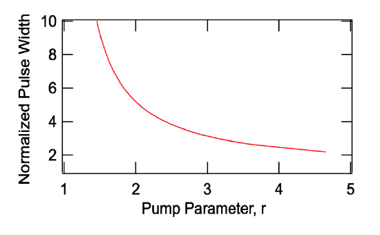
The pulse width normalized to the cavity decay time \(\tau_p\) is shown in Figure 4.14.
Passive Q-Switching
In the case of passive Q-switching the intracavity loss modulation is per- formed by a saturable absorber, which introduces large losses for low intensities of light and small losses for high intensity.
Relaxation oscillations are due to a periodic exchange of energy stored in the laser medium by the inversion and the light field. Without the saturable absorber these oscillations are damped. If for some reason there is two much gain in the system, the light field can build up quickly. Especially for a low gain cross section the backaction of the growing laser field on the inversion is weak and it can grow further. This growth is favored in the presence of loss that saturates with the intensity of the light. The laser becomes unstabile, the field intensity growth as long as the gain does not saturate below the net loss, see Fig.4.15.
Now, we want to show that the saturable absorber leads to a destabilization of the relaxation oscillations resulting in the giant pulse laser.
We extend our laser model by a saturable absorber as shown in Figure 4.16
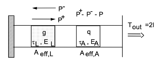
equations for a passively Q-switched laser
We make the following assumptions: First, the transverse relaxation times of the equivalent two level models for the laser gain medium and for the saturable absorber are much faster than any other dynamics in our system, so that we can use rate equations to describe the laser dynamics. Second, we assume that the changes in the laser intensity, gain and saturable absorption are small on a time scale on the order of the round-trip time \(T_R\) in the cavity, (i.e. less than 20%). Then, we can use the rate equations of the laser as derived above plus a corresponding equation for the saturable loss q similar to the equation for the gain.
\[T_R \dfrac{dP}{dt} = 2(\text{g} - l - q) P\label{eq4.4.18} \]
\[T_R \dfrac{d \text{g}}{dt} = -\dfrac{\text{g} - \text{g}_0}{T_L} - \dfrac{\text{g} T_R P}{E_L} \nonumber \]
\[T_R \dfrac{dq}{dt} = -\dfrac{q -q_0}{T_A} - \dfrac{qT_R P}{E_A}\label{eq4.4.20} \]
where \(P\) denotes the laser power, \(\text{g}\) the amplitude gain per roundtrip, \(l\) the linear amplitude losses per roundtrip, \(\text{g}_0\) the small signal gain per roundtrip and q0 the unsaturated but saturable losses per roundtrip. The quantities \(T_L = \tau_L/T_R\) and \(T_A = \tau_A/T_R\) are the normalized upper-state life- time of the gain medium and the absorber recovery time, normalized to the round-trip time of the cavity. The energies \(E_L = h \nu A_{eff,L}/2^*\sigma_L\) and \(E_A = h \nu A_{eff,A}/2^*\sigma_A\) are the saturation energies of the gain and the absorber, respectively. .
For solid state lasers with gain relaxation times on the order of \(\tau_L \approx 100 \mu s\) or more, and cavity round-trip times \(T_R \approx 10\) ns, we obtain \(T_L \approx 10^4\). Furthermore, we assume absorbers with recovery times much shorter than the round-trip time of the cavity, i.e. \(\tau_A \approx 1 - 100\) ps, so that typically \(T_A ≈ 10^{-4}\) to \(10^{-2}\). This is achievable in semiconductors and can be engineered at will by low temperature growth of the semiconductor material [20, 30]. As long as the laser is running cw and single mode, the absorber will follow the instantaneous laser power. Then, the saturable absorption can be adiabatically eliminated, by using eq.(\(\ref{eq4.4.20}\))
\[q = \dfrac{q_0}{1 + P/P_A} \text{ with } P_A = \dfrac{E_A}{\tau_A}, \nonumber \]
and back substitution into eq.(\(\ref{eq4.4.18}\)). Here, \(P_A\) is the saturation power of the absorber. At a certain amount of saturable absorption, the relaxation oscillations become unstable and Q-switching occurs. To find the stability criterion, we linearize the system
\[T_R \dfrac{dR}{dt} = (\text{g} - l -q(P))P \nonumber \]
\[T_R \dfrac{d\text{g}}{dt} = -\dfrac{\text{g} - \text{g}_0}{T_L} - \dfrac{\text{g} T_R P}{E_L}. \nonumber \]
Stationary solution
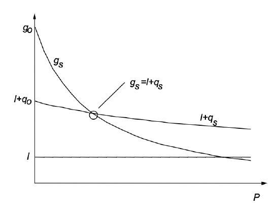
As in the case for the cw-running laser the stationary operation point of the laser is determined by the point of zero net gain
\[\begin{array} {rcl} {\text{g}_s} & = & {l + q_s} \\ {\dfrac{\text{g}_0}{1 + P_s/P_L}} & = & {l + \dfrac{q_0}{1 + P_s/P_A}.} \end{array}\label{eq4.4.24} \]
The graphical solution of this equation is shown in Figure 4.17
Stability of stationary operating point or the condition for Q-switching
For the linearized system, the coefficient matrix corresponding to Eq.(4.3.6) changes only by the saturable absorber [23]:
\[T_R \dfrac{d}{dt} \left (\begin{matrix} \Delta P_0 \\ Delta \text{g}_0 \end{matrix} \right ) = A \left (\begin{matrix} \Delta P_0 \\ Delta \text{g}_0 \end{matrix} \right ), \text{ with } A = \left (\begin{matrix} -2 \dfrac{dq}{dP}|_{cw} P_s & 2P_s \\ -\tfrac{gsT_R}{E_L} & -\tfrac{T_R}{\tau_{stim}} \end{matrix} \right )\label{eq4.4.25} \]
The coefficient matrix \(A\) does have eigenvalues with negative real part, if and only if its trace is negative and the determinante is positive which results in two conditions
\[-2P \dfrac{dq}{dP}|_{cw} < \dfrac{r}{T_L} \text{ with } r = 1 + \dfrac{P_A}{P_L} \text{ and } P_L = \dfrac{E_L}{\tau_L},\label{eq4.4.26} \]
and
\[\dfrac{dq}{dP}|_{cw} \dfrac{r}{T_L} + 2 \text{g}_s \dfrac{r - 1}{T_L} > 0. \nonumber \]
After cancelation of \(T_L\) we end up with
\[\left |\dfrac{dq}{dP} \right |_{cw} < \left |\dfrac{d\text{g}_s}{dP} \right |_{cw}\label{eq4.4.28} \]
For a laser which starts oscillating on its own, relation \(\ref{eq4.4.28}\) is automatically fulfilled since the small signal gain is larger than the total losses, see Figure 4.17. Inequality (\(\ref{eq4.4.26}\)) has a simple physical explanation. The right hand side of (\(\ref{eq4.4.26}\)) is the relaxation time of the gain towards equilibrium, at a given pump power and constant laser power. The left hand side is the decay time of a power fluctuation of the laser at fixed gain. If the gain can not react fast enough to fluctuations of the laser power, relaxation oscillations grow and result in passive Q-switching of the laser.
As can be seen from Eq.\(\ref{eq4.4.24}\) and Eq.(\(\ref{eq4.4.26}\)), we obtain
\[-2T_L P \dfrac{dq}{dP}|_{cw} = 2T_L q_0 \dfrac{\tfrac{P}{\chi P_L}}{(1 + \tfrac{P}{\chi P_L})^2}|_{cw} < r_s \text{ with } \chi = \dfrac{P_A}{P_L},\label{eq4.4.29} \]
where \(\chi\) is an effective ”stiffness” of the absorber against cw saturation. The stability relation \(\ref{eq4.4.29}\) is visualized in Figure 4.18.
Image removed due to copyright restrictions. Please see: Kaertner, Franz, et al. "Control of solid state laser dynamics by semiconductor devices." Optical Engineering 34, no. 7 (July 1995): 2024-2036.
Figure 4.18: Graphical representation of cw-Q-switching stability relation for different products \(2q_0T_L\). The cw-stiffness used for the the plots is \(\chi = 100\).
The tendency for a laser to Q-switch increases with the product \(q_0T_L\) and decreases if the saturable absorber is hard to saturate, i.e. \(\chi \gg 1\). As can be inferred from Figure 4.18 and eq.(\(\ref{eq4.4.26}\)), the laser can never Q-switch, i.e. the left side of eq.(\(\ref{eq4.4.26}\)) is always smaller than the right side, if the quantity
\[MDF = \dfrac{2q_0T_L}{\chi} < 1\label{eq4.4.27} \]
is less than 1. The abbreviation MDF stands for mode locking driving force, despite the fact that the expression (\(\ref{eq4.4.27}\)) governs the Q-switching instability. We will see, in the next section, the connection of this parameter with mode locking. For solid-state lasers with long upper state life times, already very small amounts of saturable absorption, even a fraction of a percent, may lead to a large enough mode locking driving force to drive the laser into Q-switching. Figure 4.19 shows the regions in the \(\chi\) − \(P/P_L\) - plane where Q-switching can occur for fixed MDF according to relation (\(\ref{eq4.4.26}\)). The area above the corresponding MDF-value is the Q-switching region. For MDF < 1, cw-Q-switching can not occur. Thus, if a cw-Q-switched laser has to be designed, one has to choose an absorber with a MDF >1. The further the operation point is located in the cw-Q-switching domain the more pronounced the cw-Q-switching will be. To understand the nature of the instability we look at the eigen solution and eigenvalues of the linearized equations of motion \(\ref{eq4.4.25}\)
Image removed due to copyright restrictions. Please see: Kaertner, Franz, et al. "Control of solid state laser dynamics by semiconductor devices." Optical Engineering 34, no. 7 (July 1995): 2024-2036.
Figure 4.19: For a given value of the MDF, cw-Q-switching occurs in the area above the corresponding curve. For a MDF-value less than 1 cw-Qswitching can not occur.
\[\dfrac{d}{dt} \left (\begin{matrix} \Delta P_0 (t) \\ \Delta g_0 (t) \end{matrix} \right ) = s \left (\begin{matrix} \Delta P_0 (t) \\ \Delta g_0 (t) \end{matrix} \right ) \nonumber \]
which results in the eigenvalues
\[sT_R = \dfrac{A_{11} + A_{22}}{2} \pm j \sqrt{A_{11}A_{22} - A_{12}A_{21} - \left ( \dfrac{A_{11} + A_{22}}{2} \right )^2}. \nonumber \]
With the matrix elements according to eq.(\(\ref{eq4.4.25}\)) we get
\[s = \dfrac{-\tfrac{2}{T_R} \tfrac{dq}{dP}|_{cw} P_s - \tfrac{1}{\tau_{stim}}}{2} \pm j \omega_Q \nonumber \]
\[\omega_Q = \sqrt{-\dfrac{2}{T_R} \dfrac{dq}{dP}|_{cw} P_s \dfrac{r}{\tau_L} + \dfrac{r - 1}{\tau_p \tau_L} - \left (\dfrac{-\tfrac{2}{T_R} \tfrac{dq}{dP}|_{cw} P_s - \tfrac{1}{\tau_{stim}}}{2} \right )^2} \nonumber \]
where the pump parameter is now defined as the ratio between small signal gain the total losses in steady state, i.e. \(r = g_0/(l + q_s)\). This somewhat lengthy expression clearly shows, that when the system becomes unstable, \(-2\dfrac{dq}{dP} |_{cw} P_s > \dfrac{T_R}{\tau_{stim}}\), with \(\tau_L \gg \tau_p\), there is a growing oscillation with frequency
\[\omega_Q \approx \dfrac{r - 1}{\tau_p \tau_L} \approx \dfrac{1}{\tau_p \tau_{stim}}. \nonumber \]
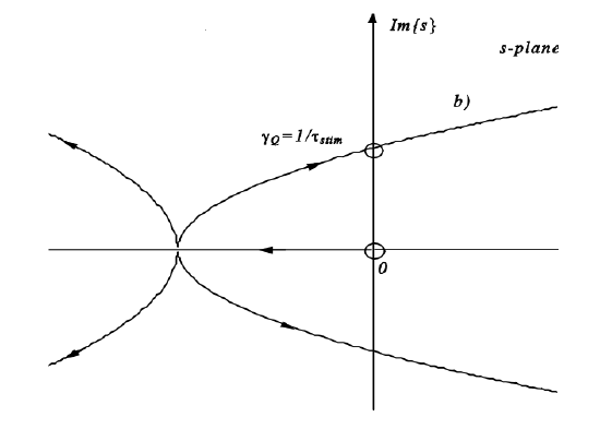
That is, passive Q-switching can be understood as a destabilization of the relaxation oscillations of the laser. If the system is only slightly in the instable regime, the frequency of the Q-switching oscillation is close to the relaxation oscillation frequency. If we define the growth rate \(\gamma_Q\), introduced by the saturable absorber as a prameter, the eigen values can be written as
\[s = \dfrac{1}{2} \left ( \gamma_Q - \dfrac{1}{\tau_{stim}} \right ) \pm j \sqrt{\gamma_Q \dfrac{r}{\tau_L} + \dfrac{r - 1}{\tau_p \tau_L} - \left (\dfrac{\gamma_Q - \tfrac{1}{\tau_{stim}}{2} \right )^2}. \nonumber \]
Figure 4.20 shows the root locus plot for a system with and without a sat- urable absorber. The saturable absorber destabilizes the relaxation oscillations. The type of bifurcation is called a Hopf bifurcation and results in an oscillation.
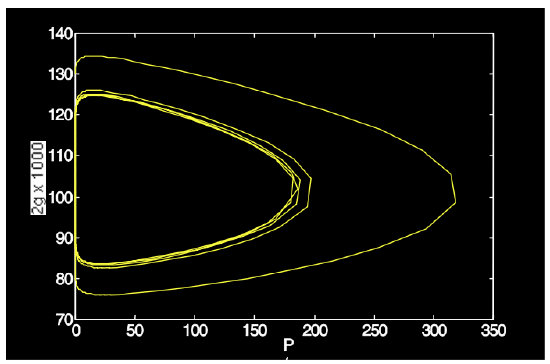
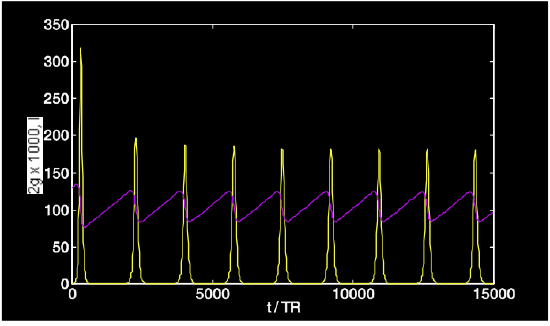
As an example, we consider a laser with the following parameters: \(\tau_L = 250 \mu s\), \(T_R = 4ns\), \(2l_0 = 0.1\), \(2q_0 = 0.005\), \(2g_0 = 2\), \(P_L/P_A = 100\). The rate equations are solved numberically and shown in Figures4.21 and 4.22.