
4.5: Example- Single Mode CW-Q-Switched Microchip Lasers
- Page ID
- 49295

Q-switched microchip lasers are compact and simple solid-state lasers, which can provide a high peak power with a diffraction limited output beam. Due to the extremely short cavity length, typically less than 1 mm, single-frequency Q-switched operation with pulse widths well below a ns can be achieved. Pulse durations of 337 ps and 218 ps have been demonstrated with a passively Q-switched microchip laser consisting of a \(\ce{Nd}: \ce{YAG}\) crystal bonded to a thin piece of \(\ce{Cr}^{4+}: \ce{YAG}\) [8, 9]. Semiconductor saturable absorbers were used to passively Q-switch a monolithic \(\ce{Nd}: \ce{YAG}\) laser producing 100 ns pulses [38].
Set-up of the Passively Q-Switched Microchip Laser
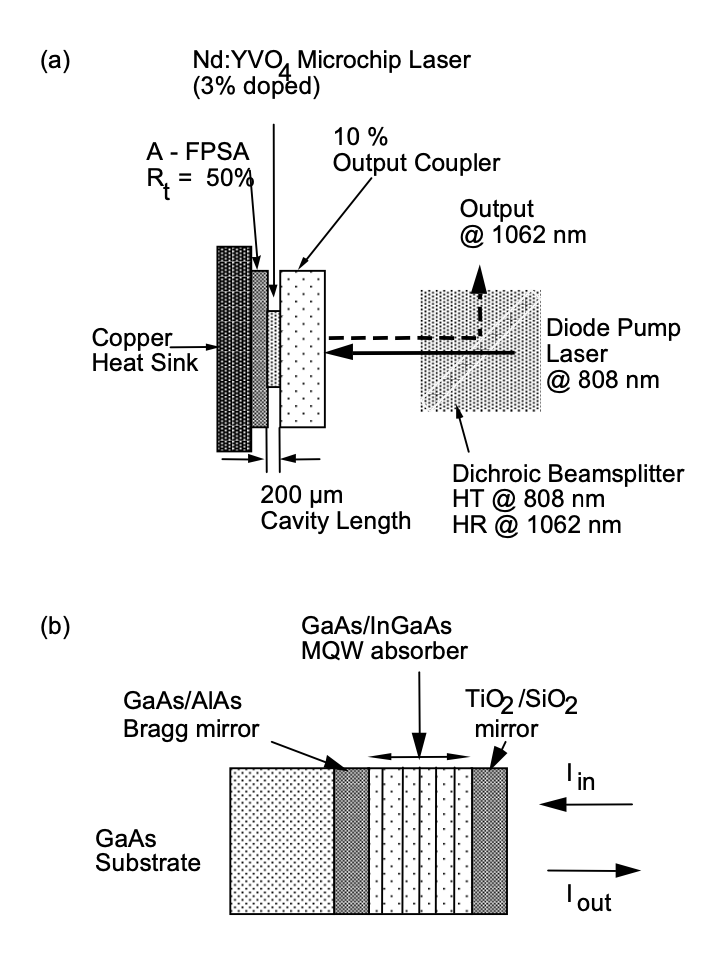
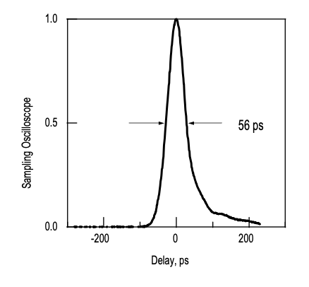
Figure 4.23(a) shows the experimental set-up of the passively Q-switched microchip laser and Figure 4.23(b) the structure of the semiconductor saturable absorber [12, 13]. The saturable absorber structure is a so called anti-resonant Fabry-Perot saturable absorber (A-FPSA), because in a microchip laser the beam size is fixed by the thermal lens that builds up in the laser crystal, when pumped with the diode laser. Thus, one can use the top reflector of the A-FPSA to scale the effective saturation intensity of the absorber with respect to the intracavity power. The 200 or 220 \(\mu\)m thick \(\ce{Nd}: \ce{YVO4}\) or \(\ce{Nd}: \ce{LaSc3(BO3)4}\), (Nd:LSB) laser crystal [39] is sandwiched be- tween a 10% output coupler and the A-FPSA. The latter is coated for high reflection at the pump wavelength of 808 nm and a predesigned reflectivity at the laser wavelength of 1.062 \(\mu\) m, respectively. The laser crystals are pumped by a semiconductor diode laser at 808 nm through a dichroic beam-splitter, that transmits the pump light and reflects the output beam at 1.064 μm for the \(\ce{Nd}: \ce{YVO4}\) or 1.062 μm for the \(\ce{Nd}:\ce{LSB}\) laser. To obtain short Q- switched pulses, the cavity has to be as short as possible. The highly doped laser crystals with a short absorption length of only about 100\(\mu\)m lead to a short but still efficient microchip laser [13]. The saturable absorber consists of a dielectric top mirror and 18 pairs of GaAs/InGaAs MQW’s grown on a GaAs/AlAs Bragg-mirror. The total optical thickness of the absorber is on the order of 1 \(\mu\)m. Therefore, the increase of the cavity length due to the absorber is neglegible. For more details see [12, 13]. Pulses as short as 56 ps, Figure (4.24), have been achieved with Nd:LSB-crystals.
Dynamics of a Q-Switched Microchip Laser
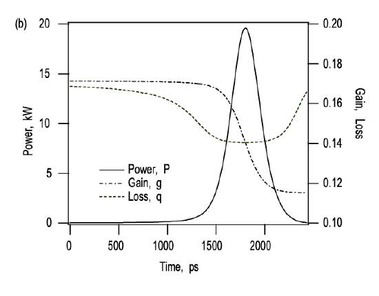
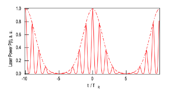
The passively Q-switched microchip laser, shown in Figure 4.23(a), is perfectly modelled by the rate equations (4.4.18) to (4.4.20). To understand the basic dependence of the cw-Q-switching dynamics on the absorber parameters, we performed numerical simulations of the \(\ce{Nd}: \ce{LSB}\) microchip laser, as shown in Figure 4.23. The parameter set used, is given in Table 4.2. For these parameters, we obtain according to eq.(4.4.24) a mode locking driving force of MDF = 685. This laser operates clearly in the cw-Q-switching regime as soon as the laser is pumped above threshold. Note, the Q-switching condition (4.4.30) has only limited validity for the microchip laser considered here, because, the cavity length is much shorter than the absorber recovery time. Thus the adiabatic elimination of the absorber dynamics is actually not any longer justified. Figures 4.25 and 4.26 show the numerical solution of the set of rate equations (4.4.18) to (4.4.20) on a microsecond timescale and a picosecond timescale close to one of the pulse emission events.
| Parameter | value |
| 2 \(g_0\) | 0.7 |
| 2 \(q_0\) | 0.03 |
| 2 \(l\) | 0.14 |
| \(T_R\) | 2.7 ps |
| \(\tau_L\) | 87 \(\mu\) s |
| \(\tau_A\) | 24 ps |
| \(E_L\) | 20 \(\mu\) J |
| \(E_A\) | 7.7 nJ |
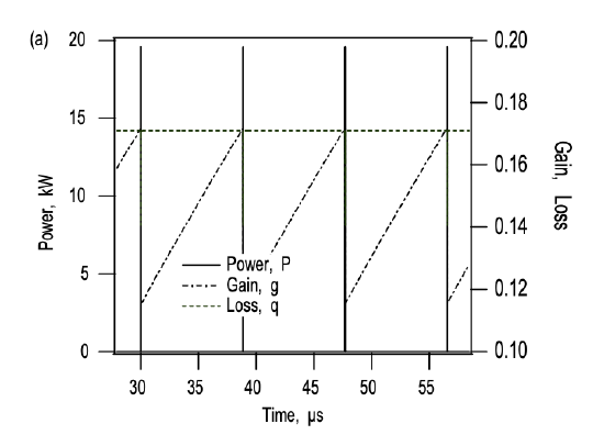
No analytic solution to the set of rate equations is known. Therefore, optimization of Q-switched lasers has a long history [4, 5], which in general results in complex design criteria [5], if the most general solution to the rate equations is considered. However, a careful look at the simulation results leads to a set of very simple design criteria, as we show in the following. As seen from Figure 4.25, the pulse repetition time \(T_{rep}\) is many orders of magnitude longer than the width of a Q-switched pulse. Thus, between two pulse emissions, the gain increases due to pumping until the laser reaches threshold. This is described by eq.(4.4.19), where the stimulated emission term can be neglected. Therfore, the pulse repetition rate is determined by the relation that the gain has to be pumped to threshold again \(g_{th} = l + q_0\), if it is saturated to the value gf after pulse emission. In good approximation, \(g_f = l - q_0\), as long as it is a positive quantity. If \(T_{rep} < \tau_L\), one can linearize the exponential and we obtain
\[g_{th} - g_f = g_0 \dfrac{T_{rep}}{\tau_L} \nonumber \]
\[T_{rep} = \tau_L \dfrac{g_{th} - g_f}{g_0} = \tau_L \dfrac{2q_0}{g_0}. \nonumber \]
Figure 4.26 shows, that the power increases, because, the absorber saturates faster than the gain. To obtain a fast raise of the pulse, we assume an absorber which saturates much easier than the gain, i.e. \(E_A \ll E_L\), and the recovery times of gain and absorption shall be much longer than the pulse width \(\tau_{pulse}\), \(\tau_{A} \gg \tau_{pulse}\). Since, we assume a slow gain and a slow absorber, we can neglect the relaxation terms in eqs.(4.4.19) and (4.4.20) during growth and decay of the pulse. Then the equations for gain and loss as a function of the unknown Q-switched pulse shape \(f_Q (t)\)
\[P(t) = E_P f_Q (t) \nonumber \]
can be solved. The pulse shape \(f_Q (t)\) is again normalized, such that its integral over time is one and \(E_P\) is, therefore, the pulse energy. Analogous to the derivation for the Q-switched mode locking threshold in eqs.(4.6.3) and (4.6.4), we obtain
\[q(t) = q_0 \exp \left [ -\dfrac{E_P}{E_A} \int_{-\infty}^{t} f_Q (t') dt' \right ],\label{eq4.5.4} \]
\[g(t) = g_{th} \exp \left [ -\dfrac{E_P}{E_A} \int_{-\infty}^{t} f_Q (t') dt' \right ],\label{eq4.5.5} \]
Substitution of these expressions into the eq.(4.4.18) for the laser power, and integration over the pulse width, determines the extracted pulse energy. The result is a balance between the total losses and the gain.
\[l + q_P (E_P) = g_P (E_P)\label{eq4.5.6} \]
with
\[q_P (E_P) = q_0 \dfrac{1 - \exp [-\tfrac{E_P}{E_A}]}{\tfrac{E_P}{E_A}}, \nonumber \]
\[g_P (E_P) = g_{th} \dfrac{1 - \exp [-\tfrac{E_P}{E_A}]}{\tfrac{E_P}{E_A}}, \nonumber \]
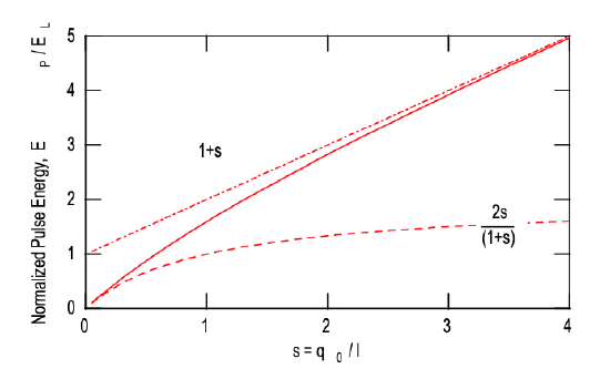
Because, we assumed that the absorber is completely saturated, we can set \(q_P (E_P) \approx 0\). Figure 4.27 shows the solution of eq.(\(\ref{eq4.5.6}\)), which is the pulse energy as a function of the ratio between saturable and nonsaturable losses \(s = q_0/l\). Also approximate solutions for small and large s are shown as the dashed curves. Thus, the larger the ratio between saturable and nonsaturable losses is, the larger is the intracavity pulse energy, which is not surprising. Note, the extracted pulse energy is proportional to the output coupling, which is \(2l\) if no other losses are present. If we assume, \(s \ll 1\), then, we can use approximately the low energy approximation
\[E_P = 2 E_L \dfrac{q_0}{l + q_0}. \nonumber \]
The externally emitted pulse energy is then given by
\[E_P^{ex} = 2l E_P = E_L \dfrac{4l q_0}{l + q_0}.\label{eq4.5.10} \]
Thus, the total extracted pulse energy is completely symmetric in the saturable and non saturable losses. For a given amount of saturable absorption, the extracted pulse energy is maximum for an output coupling as large as possible. Of course threshold must still be reached, i.e. \(l + q_0 < g_0\). Thus, in the following, we assume \(l > q_0\) as in Figure 4.26. The absorber is immediatelly bleached, after the laser reaches threshold. The light field growth and extracts some energy stored in the gain medium, until the gain is saturated to the low loss value \(l\). Then the light field decays again, because the gain is below the loss. During decay the field can saturate the gain by a similar amount as during build-up, as long as the saturable losses are smaller than the constant output coupler losses l, which we shall assume in the following. Then the pulse shape is almost symmetric as can be seen from Figure 4.26(b) and is well approximated by a secant hyperbolicus square for reasons that will become obvious in a moment. Thus, we assume
\[f_Q (t) = \dfrac{1}{2 \tau_P} \text{sech}^2 \left (\dfrac{t}{\tau_p} \right ). \nonumber \]
With the assumption of an explicite pulse form, we can compute the pulse width by substitution of this ansatz into eq.(4.4.18) and using (\(\ref{eq4.5.4}\)), (\(\ref{eq4.5.5}\))
\[-\dfrac{2T_R}{\tau_P} \tanh \left (\dfrac{t}{\tau_p} \right ) = g_{th} \exp \left [ \right ] - l. \nonumber \]
Again, we neglect the saturated absorption. If we expand this equation up to first order in \(E_P/E_L\) and compare coefficients, we find from the constant term the energy (\(\ref{eq4.5.10}\)), and from the tanh-term we obtain the following simple expression for the pulse width
\[\tau_P = 2 \dfrac{T_R}{q_0}. \nonumber \]
For the FWHM pulse width of the resulting \(\text{sech}^2\)-pulse we obtain
\[\tau_{P,FWHM} = 3.5 \dfrac{T_R}{q_0}.\label{eq4.5.14} \]
Thus, for optimium operation of a Q-switched microchip laser, with respect to minimum pulse width and maximum extracted energy in the limits considered here, we obtain a very simple design criterium. If we have a maximum small signal round-trip gain g0, we should design an absorber with q0 somewhat smaller than \(g_0/2\) and an output coupler with \(q_0 < l < g_0 - q_0\), so that the laser still fullfills the cw-Q-switching condition. It is this simple optimization, that allowed us to reach the shortest pulses every generated from a cw-Q-switched solid-state laser. Note, for a maximum saturable absorption of \(2\ q_0 = 13%\), a cavity roundtip time of \(T_R = 2.6\) ps for the \(\ce{Nd}: \ce{YVO4}\) laser, one expects from (\(\ref{eq4.5.14}\)) a pulse width of about \(\tau_P = 70ps\), which is close to what we observed in the experiment above. We achieved pulses between 56 and 90 ps [13]. The typical extracted pulse energies were on the order of \(E_P = 0.1 - 0.2 \mu J\) for pulses of about 60\(ps\) [13]. Using a saturation energy of about \(E_L = 30\ \mu J\) and an output coupler loss of \(2l = 0.1\), we expect, according to (\(\ref{eq4.5.10}\)), a maximum extracted pulse energy of \(E_P^{ex} = 2\ \mu J\). Thus, we have a deviation of one order of magnitude, which clearly indicates that the absorber still introduces too much of nonsaturable intracavity losses. Lowering of these losses should lead to \(\mu J\) - 50 ps pulses from this type of a very simple and cheap laser, when compared with any other pulse generation technique.