7.1: Kerr-Lens Mode Locking (KLM)
- Page ID
- 44665

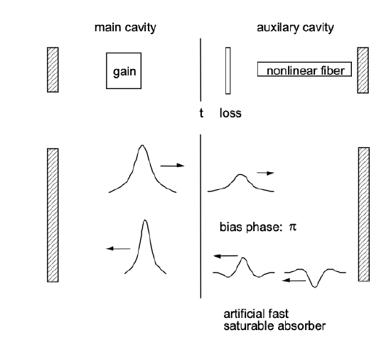
The general principle behind Kerr-Lens Mode Locking is sketched in Figure 7.1. A pulse that builds up in a laser cavity containing a gain medium and a Kerr medium experiences not only self-phase modulation but also self focussing, that is nonlinear lensing of the laser beam, due to the nonlinear refractive index of the Kerr medium. A spatio-temporal laser pulse propagating through the Kerr medium has a time dependent mode size as higher intensities acquire stronger focussing. If a hard aperture is placed at the right position in the cavity, it strips of the wings of the pulse, leading to a shortening of the pulse. Such combined mechanism has the same effect as a saturable absorber. If the electronic Kerr effect with response time of a few femtoseconds or less is used, a fast saturable absorber has been created. Instead of a separate Kerr medium and a hard aperture, the gain medium can act both as a Kerr medium and as a soft aperture (i.e. increased gain instead of saturable absorption). The sensitivity of the laser mode size on additional nonlinear lensing is drastically enhanced if the cavity is operated close to the stability boundary of the cavity. Therefore, it is of prime importance to understand the stability ranges of laser resonators. Laser resonators are best understood in terms of paraxial optics [11][12][14][13][15].
Review of Paraxial Optics and Laser Resonator Design
The solutions to the paraxial wave equation, which keep their form during propagation, are the Hermite-Gaussian beams. Since we consider only the fundamental transverse modes, we are dealing with the Gaussian beam
\[U(r, z) = \dfrac{U_o}{q(z)} \exp \left [ -jk \dfrac{r^2}{2q(z)} \right ], \nonumber \]
with the complex q-parameter \(q = a+jb\) or its inverse
\[\dfrac{1}{q(z)} = \dfrac{1}{R(z)} - j\dfrac{\lambda}{\pi w^2(z)}. \nonumber \]
The Gaussian beam intensity \(I(z, r) = |U(r, z)|^2\) expressed in terms of the power \(P\) carried by the beam is given by
\[I(r, z) = \dfrac{2P}{\pi w^2(z)} \exp \left [-\dfrac{2r^2}{w^2 (z)} \right ]. \nonumber \]
The use of the q-parameter simplifies the description of Gaussian beam propagation. In free space propagation from \(z_1\) to \(z_2\), the variation of the beam parameter \(q\) is simply governed by
\[q_2 = q_1 + z_2 - z_1, \nonumber \]
where \(q_2\) and \(q_1\) are the beam parameters at \(z_1\) and \(z_2\). If the beam waist, at which the beam has a minimum spot size \(w_0\) and a planar wavefront (\(R = \infty\)), is located at \(z = 0\), the variations of the beam spot size and the radius of curvature are explicitly expressed as
\[w(z) = w_o \left [1 + \left (\dfrac{\lambda z}{\pi w_o^2} \right )^2 \right ]^{1/2}, \nonumber \]
and
\[R(z) = z \left [1 + \left (\dfrac{\pi w_o^2}{\lambda z} \right )^2 \right ]. \nonumber \]
The angular divergence of the beam is inversely proportional to the beam waist. In the far field, the half angle divergence is given by,
\[\theta = \dfrac{\lambda}{\pi w_o}, \nonumber \]
as illustrated in Figure 7.2.
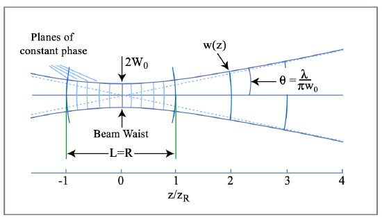
Figure by MIT OCW.
Due to diffraction, the smaller the spot size at the beam waist, the larger the divergence. The Rayleigh range is defined as the distance from the waist over which the beam area doubles and can be expressed as
\[z_R = \dfrac{\pi w_o^2}{\lambda}. \nonumber \]
The confocal parameter of the Gaussian beam is defined as twice the Rayleigh range
\[b = 2 z_R = \dfrac{2\pi w_o^2}{\lambda}, \nonumber \]
and corresponds to the length over which the beam is focused. The propagation of Hermite-Gaussian beams through paraxial optical systems can be efficiently evaluated using the ABCD-law [11]
\[q_2 = \dfrac{Aq_1 + B}{Cq_1 + D}\label{eq7.1.10} \]
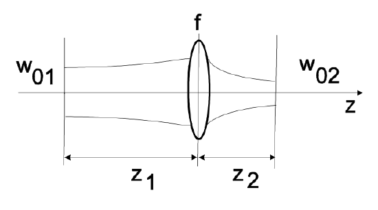
where \(q_1\) and \(q_2\) are the beam parameters at the input and the output planes of the optical system or component. The ABCD matrices of some optical elements are summarized in Table 7.1. If a Gaussian beam with a waist \(w_{01}\) is focused by a thin lens a distance \(z_1\) away from the waist, there will be a new focus at a distance
\[z_2 = f + \dfrac{(z_1 - f) f^2}{(z_1 - f)^2 + (\tfrac{\pi w_{01}^2}{\lambda})^2}, \nonumber \]
and a waist \(w_{02}\)
\[\dfrac{1}{w_{02}^2} = \dfrac{1}{w_{01}^2} \left (1 - \dfrac{z_1}{f} \right )^2 + \dfrac{1}{f^2} \left (\dfrac{\pi w_{01}}{\lambda} \right )^2 \nonumber \]
Two-Mirror Resonators
We consider the two mirror resonator shown in Figure 7.4.
| Optical Element | ABCD-Matrix |
|---|---|
| Free Space Distance \(L\) | \(\left (\begin{matrix} 1 & L \\ 0 & 1 \end{matrix} \right)\) |
| Thin Lens with focal length \(f\) | \(\left (\begin{matrix} 1 & 0 \\ -1/f & 1 \end{matrix} \right )\) |
| Mirror under Angle \(\theta\) to Axis and Radius \(R\) Sagittal Plane | \(\left (\begin{matrix} 1 & 0 \\ \tfrac{-2 \cos \theta}{R} & 1 \end{matrix} \right )\) |
| Mirror under Angle \(\theta\) to Axis and Radius \(R\) Tangential Plane | \(\left (\begin{matrix} 1 & 0 \\ \tfrac{-2}{R\cos \theta} & 1 \end{matrix} \right)\) |
| Brewster Plate under Angle \(\theta\) to Axis and Thickness \(d\), Sagittal Plane | \(\left (\begin{matrix} 1 & \tfrac{d}{n} \\ 0 & 1 \end{matrix} \right)\) |
| Brewster Plate under Angle \(\theta\) to Axis and Thickness \(d\), Tangential Plane | \(\left (\begin{matrix} 1 & \tfrac{d}{n^3} \\ 0 & 1 \end{matrix} \right)\) |
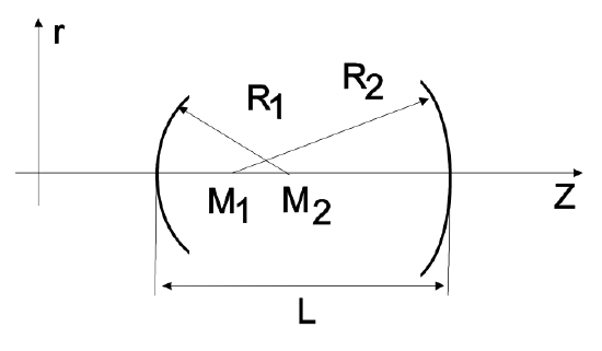
The resonator can be unfolded for an ABCD-matrix analysis, see Figure 7.5.
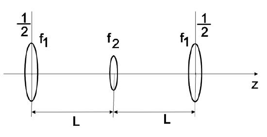
The product of ABCD matrices describing one roundtrip according to Figure 7.5 are then given by
\[M = \left ( \begin{matrix} 1 & 0 \\ \tfrac{-1}{2f_1} & 1 \end{matrix} \right) \left (\begin{matrix} 1 & L \\ 0 & 1 \end{matrix} \right ) \left (\begin{matrix} 1 & 0 \\ \tfrac{-1}{f_2} & 1 \end{matrix} \right) \left (\begin{matrix} 1 & L \\ 0 & 1 \end{matrix} \right) \left (\begin{matrix} 1 & 0 \\ \tfrac{-1}{2f_1} & 1 \end{matrix} \right) \nonumber \]
where \(f_1 = R_1/2\), and \(f_2 = R_2/2\). To carry out this product and to formulate the cavity stability criteria, it is convenient to use the cavity parameters \(g_i = 1 - L/R_i\), \(i = 1,2\). The resulting cavity roundtrip ABCD-matrix can be written in the form
\[M = \left (\begin{matrix} (2g_1g_2 - 1) & 2g_2L \\ 2g_1(g_1 g_2 - 1)/L & (2g_1g_2 - 1) \end{matrix} \right) = \left (\begin{matrix} A & B \\ C & D \end{matrix} \right). \nonumber \]
Resonator Stability
The ABCD matrices describe the dynamics of rays propagating inside the resonator. An optical ray is characterized by the vector \(r = \left ( \begin{matrix} r \\ r' \end{matrix} \right )\), where \(r\) is the distance from the optical axis and \(r'\) the slope of the ray to the optical axis. The resonator is stable if no ray escapes after many round-trips, which is the case when the eigenvalues of the matrix \(M\) are less than one. Since we have a lossless resonator, i.e. \(\text{det}|M| = 1\), the product of the eigenvalues has to be 1 and, therefore, the stable resonator corresponds to the case of a complex conjugate pair of eigenvalues with a magnitude of 1. The eigenvalue equation to \(M\) is given by
\[\text{det} |M - \lambda \cdot 1| = \text{det} \left |\left (\begin{matrix} (2g_1 g_2 - 1) - \lambda & 2g_2 L \\ 2g_1(g_1g_2 - 1)/L & (2g_1 g_2 - 1) - \lambda \end{matrix} \right ) \right | = 0,\label{eq7.1.15} \]
\[\lambda^2 - 2(2g_1g_2 - 1) \lambda + 1 = 0. \nonumber \]
The eigenvalues are
\[\lambda_{1/2} = (2g_1g_2 - 1) \pm \sqrt{(2g_1g_2 - 1)^2 - 1}, \nonumber \]
\[= \begin{cases} \exp (\pm \theta), \text{cosh} \theta = 2g_1 g_2 - 1, & \text{ for } |2g_1 g_2 - 1| > 1 \\ \exp (\pm j \psi), \text{cos} \psi = 2g_1 g_2 - 1, & \text{ for } |2g_1 g_2 - 1| \le 1 \end{cases} \nonumber \]
The case of a complex conjugate pair with a unit magnitude corresponds to a stable resontor. Therfore, the stability criterion for a stable two mirror resontor is
\[|2g_1g_2 - 1| \le 1. \nonumber \]
The stable and unstable parameter ranges are given by
\[\text{stable : } 0 \le g_1 \cdot g_2 = S \le 1 \nonumber \]
\[\text{unstable : } g_1 g_2 \le 0; \text{ or } g_1 g_2 \ge 1. \nonumber \]
where \(S = g_1 \cdot g_2\), is the stability parameter of the cavity. The stabil- ity criterion can be easily interpreted geometrically. Of importance are the distances between the mirror mid-points \(M_i\) and cavity end points, i.e. \(g_i = (R_i - L)/R_i = -S_i/R_i\), as shown in Figure 7.6.
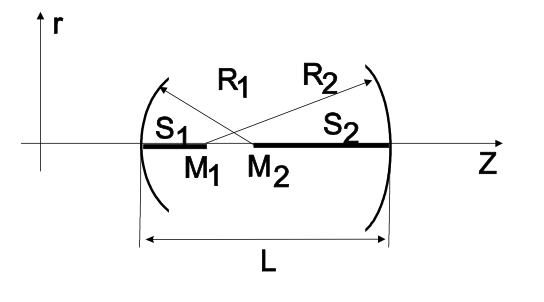
The following rules for a stable resonator can be derived from Figure 7.6 using the stability criterion expressed in terms of the distances \(S_i\). Note, that the distances and radii can be positive and negative
\[\text{stable: } 0 \le \dfrac{S_1S_2}{R_1R_2} \le 1. \nonumber \]
The rules are:
• A resonator is stable, if the mirror radii, laid out along the optical axis, overlap.
• A resonator is unstable, if the radii do not overlap or one lies within the other.
Figure 7.7 shows stable and unstable resonator configurations.
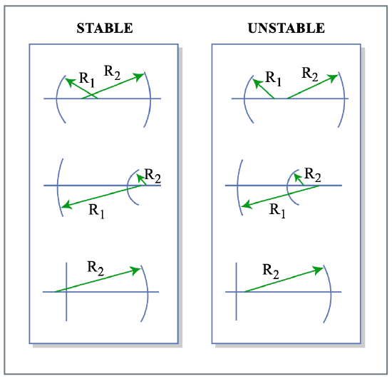
Figure by MIT OCW.
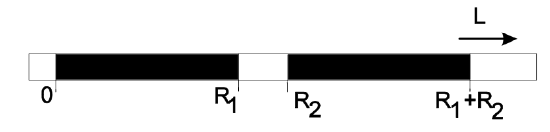
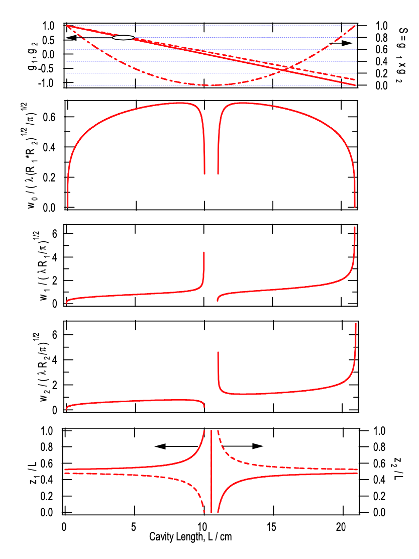
For a two-mirror resonator with concave mirrors and \(R_1 \le R_2\), we obtain the general stability diagram as shown in Figure 7.8. There are two ranges for the mirror distance \(L\), within which the cavity is stable, \(0 \le L \le R_1\) and \(R_2 \le L \le R_1 + R_2\). It is interesting to investigate the spot size at the mirrors and the minimum spot size in the cavity as a function of the mirror distance \(L\).
Resonator Mode Characteristics
The stable modes of the resonator reproduce themselves after one round-trip, i.e. from Eq.(\(\ref{eq7.1.10}\)) we find
\[q_1 = \dfrac{Aq_1 + B}{Cq_1 + D} \nonumber \]
The inverse q-parameter, which is directly related to the phase front curvature and the spot size of the beam, is determined by
\[\left (\dfrac{1}{q} \right )^2 + \dfrac{A - D}{B} \left (\dfrac{1}{q} \right ) + \dfrac{1 - AD}{B^2} = 0. \nonumber \]
The solution is
\[\left (\dfrac{1}{q} \right )_{1/2} = -\dfrac{A - D}{2B} \pm \dfrac{j}{2|B|} \sqrt{(A + D)^2 - 1} \nonumber \]
If we apply this formula to (\(\ref{eq7.1.15}\)), we find the spot size on mirror 1
\[\left (\dfrac{1}{q} \right )_{1/2} = - \dfrac{j}{2|B|} \sqrt{(A + D)^2 - 1} = -j \dfrac{\lambda}{\pi w_1^2}. \nonumber \]
or
\[w_1^4 = \left ( \dfrac{2\lambda L}{\pi} \right )^2 \dfrac{g_2}{g_1} \dfrac{1}{1 - g_1 g_2}\label{eq7.1.27} \]
\[= \left ( \dfrac{\lambda R_1}{\pi} \right )^2 \dfrac{R_2 - L}{R_1 - L} \left ( \dfrac{L}{R_1 + R_2 - L} \right ). \nonumber \]
By symmetry, we find the spot size on mirror 3 via switching index 1 and 2:
\[w_2^4 = \left (\dfrac{2\lambda L}{\pi} \right )^2 \dfrac{g_1}{g_2} \dfrac{1}{1 - g_1g_2} \nonumber \]
\[= \left ( \dfrac{\lambda R_2}{\pi} \right )^2 \dfrac{R_1 - L}{R_2 - L} \left ( \dfrac{L}{R_1 + R_2 - L} \right ). \nonumber \]
The intracavity focus can be found by transforming the focused Gaussian beam with the propagation matrix
\[\begin{array} {rcl} {M} & = & {\left (\begin{matrix} 1 & z_1 \\ 0 & 1 \end{matrix} \right ) \left (\begin{matrix} 1 & 0 \\ \tfrac{-1}{2f_1} & 1 \end{matrix} \right )} \\ {} & = & {\left (\begin{matrix} 1 - \tfrac{z_1}{2f_1} & \tfrac{-1}{2f_1} \\ 0 & 1 \end{matrix} \right ),} \end{array} \nonumber \]
to its new focus by properly choosing \(z_1\), see Figure 7.9.
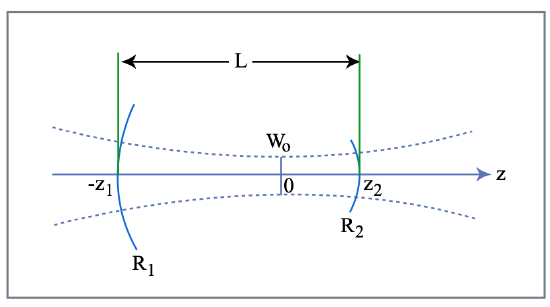
Figure by MIT OCW.
A short calculation results in
\[z_1 = L \dfrac{g_2(g_1 - 1)}{2g_1 g_2 - g_1 - g_2} \nonumber \]
\[= \dfrac{L(L - R_2)}{2L - R_1 - R_2}, \nonumber \]
and, again, by symmetry
\[z_2 = L \dfrac{g_1(g_2 - 1)}{2g_1 g_2 - g_1 - g_2} \nonumber \]
\[= \dfrac{L(L - R_1)}{2L - R_1 - R_2} = L - z_1, \nonumber \]
The spot size in the intracavity focus is
\[w_0^4 = \left (\dfrac{\lambda L}{\pi} \right )^2 \dfrac{g_1 g_2 (1 - g_1 g_2)}{(2g_1g_2 - g_1 - g_2)^2} \nonumber \]
\[= \left (\dfrac{\lambda }{\pi} \right )^2 \dfrac{L(R_1 - L)(R_2 - L)(R_1 + R_2 - L)}{(R_1 + R_2 - 2L)^2}.\label{eq7.1.37} \]
All these quantities for the two-mirror resonator are shown in Figure 7.11. Note, that all resonators and the Gaussian beam are related to the confocal resonator as shown in Figure 7.10.
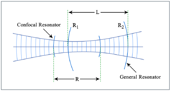
Figure by MIT OCW.
Four-Mirror Resonators
More complex resonators, like the four-mirror resonator depicted in Figure 7.12 a) can be transformed to an equivalent two-mirror resonator as shown in Figure 7.4 b) and c)
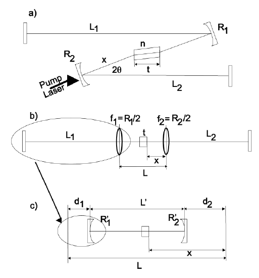
Each of the resonator arms (end mirror, \(L_1\), \(R_1\)) or (end mirror, \(L_2\), \(R_2\)) is equivalent to a new mirror with a new radius of curvature \(R_{1/2}'\) positioned a distance \(d_{1/2}\) away from the old reference plane [12]. This follows simply from the fact that each symmetric optical system is equivalent to a lens positioned at a distance \(d\) from the old reference plane
\[\begin{array} {rcl} {M} & = & {\left ( \begin{matrix} A & B \\ C & A \end{matrix} \right ) = \left ( \begin{matrix} 1 & d \\ 0 & 1 \end{matrix} \right ) \left ( \begin{matrix} 1 & 0 \\ \tfrac{-1}{f} & 1 \end{matrix} \right ) \left ( \begin{matrix} 1 & d \\ 0 & 1 \end{matrix} \right )} \\ {} & = & {\left ( \begin{matrix} 1 - \tfrac{d}{f} & d(2 - \tfrac{d}{f}) \\ \tfrac{-1}{f} & 1 - \tfrac{d}{f} \end{matrix} \right )}\end{array} \nonumber \]
with
\[\begin{array} {rcl} {d} & = & {\dfrac{A - 1}{C}} \\ {\dfrac{-1}{f}} & = & {C} \end{array} \nonumber \]
The matrix of the resonator arm 1 is given by
\[M = \left ( \begin{matrix} 1 & 0 \\ \tfrac{-2}{R_1} & 1 \end{matrix} \right ) \left ( \begin{matrix} 1 & 2L_1 \\ 0 & 1 \end{matrix} \right ) \left ( \begin{matrix} 1 & 0 \\ \tfrac{-2}{R_1} & 1 \end{matrix} \right ) = \left ( \begin{matrix} 1 - \tfrac{4L_1}{R_1} & 2L_1 \\ \tfrac{-4}{R_1} (1-\tfrac{2L_1}{R_1}) & 1-\tfrac{4L_1}{R_1} \end{matrix} \right ) \nonumber \]
from which we obtain
\[d_1 = -\dfrac{R_1}{2} \dfrac{1}{1 - R_1/(2L_1)}, \nonumber \]
\[R_1' = - \left ( \dfrac{R_1}{2} \right )^2 \dfrac{1}{L_1 [1 - R_1/(2L_1)]}. \nonumber \]
For arm lengths \(L_{1/2}\) much larger than the radius of curvature, the new radius of curvature is roughly by a factor of \(\tfrac{R_1}{4L_1}\) smaller. Typical values are \(R_1 = 10\) cm and \(L_1 = 50\) cm. Then the new radius of curvature is \(R_1' = 5\) mm. The analogous equations apply to the other resonator arm
\[d_2 = -\dfrac{R_2}{2} \dfrac{1}{1 - R_2/(2L_2)}, \nonumber \]
\[R_2' = -\left ( \dfrac{R_2}{2} \right )^2 \dfrac{1}{L_2 [1 - R_2/(2L_2)]}. \nonumber \]
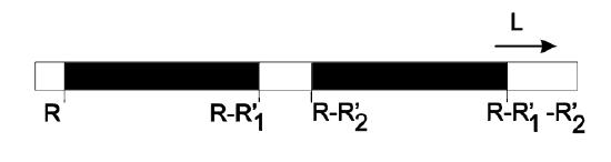
Note that the new mirror radii are negative for \(R_i/L_i < 1\). The new distance \(L'\) between the equivalent mirrors is then also negative over the region where the resonator is stable, see Fig.7.8. We obtain
\[L'= L + d_1 + d_2 = L - \dfrac{R_1 + R_2}{2} - \delta \nonumber \]
\[\delta = \dfrac{R_1}{2} \left [\dfrac{1}{1 - R_1/(2L_1)} - 1 \right ] + \dfrac{R_2}{2} \left [\dfrac{1}{1 - R_2/(2L_2)} - 1\right ] \nonumber \]
\[=-(R_1' + R_2') \nonumber \]
or
\[L = \dfrac{R_1 + R_2}{2} - (R_1' + R_2') + L' \nonumber \]
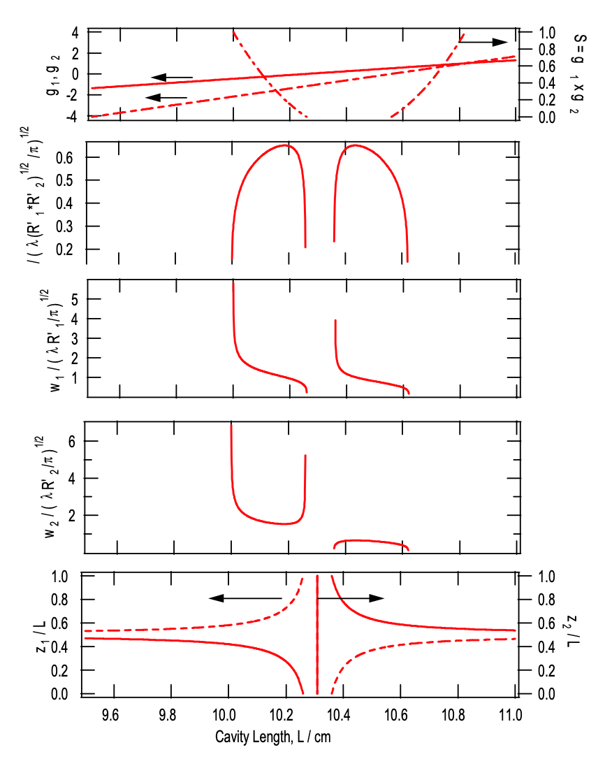
From the discussion in section 7.1.2, we see that the stability ranges cover at most a distance \(\delta\). Figure 7.13 shows the resonator characteristics as a function of the cavity length \(L\) for the following parameters \(R_1 = R_2 = 10\) cm and \(L_1 =100\) cm and \(L_2 =75\) cm, which lead to
\[\begin{array} {rcl} {d_1} & = & {-5.26\ cm} \\ {R_1'} & = & {-0.26\ cm}\end{array}\label{eq7.1.49} \]
\[\begin{array} {rcl} {d_2} & = & {-5.36\ cm} \\ {R_2'} & = & {-0.36\ cm}\end{array} \nonumber \]
\[L' = L - 10.62\ cm\label{eq7.1.51} \]
Note, that the formulas (\(\ref{eq7.1.27}\)) to (\(\ref{eq7.1.37}\)) can be used with all quantities replaced by the corresponding primed quantities in Eq.(\(\ref{eq7.1.49}\)) - (\(\ref{eq7.1.51}\)). The result is shown in Figure 7.13. The transformation from \(L\) to \(L'\) transforms the stability ranges according to Figure 7.14. The confocal parameter of the laser mode is approximately equal to the stability range.
Astigmatism Compensation
So far, we have considered the curved mirrors under normal incidence. In a real cavity this is not the case and one has to analyze the cavity performance for the tangential and sagittal beam separately. The gain medium, usually a thin plate with a refractive index \(n\) and a thickness \(t\), generates astigmatism. Astigmatism means that the beam foci for sagittal and tangential plane are not at the same position. Also, the stablity regions of the cavity are different for the different planes and the output beam is elliptical. This is so, because a beam entering a plate under an angle refracts differently in both planes, as described by different ABCD matricies for tangential and sagittal plane, see Table 7.1.Fortunately, one can balance the astigmatism of the beam due to the plate by the astigmatism introduced by the curved mirrors at a specific incidence angle \(\theta\) on the mirrors [12]. The focal length of the curved mirrors under an angle are given by
\[\begin{array} {rcl} {f_s} & = & {f/cos \theta} \\ {f_t} & = & {f \cdot cos \theta} \end{array} \nonumber \]
The propagation distance in a plate with thickness t under Brewster’s angle is given by \(t\sqrt{n^2 + 1}/n\). Thus, the equivalent traversing distances in the sagittal and the tangential planes are (Table 7.1),
\[\begin{array} {rcl} {d_s} & = & {t\sqrt{n^2 + 1} /n^2} \\ {d_f} & = & {t \sqrt{n^2 + 1} /n^4} \end{array} \nonumber \]
The different distances have to compensate for the different focal lengths in the sagittal and tangential planes. Assuming two idential mirrors \(R = R_1 = R_2\), leads to the condition
\[d_s - 2f_s = d_t - 2f_t. \nonumber \]
With \(f = R/2\) we find
\[R\sin \theta \tan \theta = Nt, \text{where } N = \sqrt{n^2 + 1} \dfrac{n^2 - 1}{n^4} \nonumber \]
Note, that \(t\) is the thickness of the plate as opposed to the path length of the beam in the plate. The equation gives a quadratic equation for \(\cos \theta\)
\[\cos^2 \theta + \dfrac{Nt}{R} \cos \theta - 1 = 0 \nonumber \]
\[\cos \theta_{1/2} = - \dfrac{Nt}{2R} \pm \sqrt{1 + \left (\dfrac{Nt}{2R} \right )^2} \nonumber \]
Since the angle is positive, the only solution is
\[\theta = \text{arccos} \left [ \sqrt{1 + \left (\dfrac{Nt}{2R} \right )^2} - \dfrac{Nt}{2R}\right ]. \nonumber \]
This concludes the design and analysis of the linear resonator.
Kerr Lensing Effects
At high intensities, the refractive index in the gain medium becomes intensity dependent
\[n = n_0 + n_2I. \nonumber \]
The Gaussian intensity profile of the beam creates an intensity dependent index profile
\[I(r) = \dfrac{2P}{\pi w^2} \exp [-2 (\dfrac{r}{w})^2 ]. \nonumber \]
In the center of the beam the index can be appoximated by a parabola
\[n(r) = n_0' (1 - \dfrac{1}{2} \gamma^2 r^2 ), \text{where} \nonumber \]
\[n_0' = n_0 + n_2 \dfrac{2P}{\pi w^2}, \gamma = \dfrac{1}{w^2} \sqrt{\dfrac{8n_2P}{n_0'\pi}}. \nonumber \]
A thin slice of a parabolic index medium is equivalent to a thin lens. If the parabolic index medium has a thickness \(t\), then the ABCD matrix describing the ray propagation through the medium at normal incidence is [16]
\[M_K = \left (\begin{matrix}\cos \gamma t & \tfrac{1}{n_0' \gamma} \sin \gamma t \\ -n_0' \gamma \sin \gamma t & \cos \gamma t \end{matrix} \right ). \nonumber \]
Note that, for small \(t\), we recover the thin lens formula (\(t \to 0\), but \(n_0'\gamma^2 t = 1/f = \text{ const}\).). If the Kerr medium is placed under Brewster’s angle, we again have to differentiate between the sagittal and tangential planes. For the sagittal plane, the beam size entering the medium remains the same, but for the tangential plane, it opens up by a factor \(n_0'\)
\[\begin{array} {rcl} {w_s} & = & {w} \\ {w_t} & = & {w \cdot n_0'} \end{array} \nonumber \]
The spotsize propotional to \(w^2\) has to be replaced by \(w^2 =w_sw_t\).Therefore, under Brewster angle incidence, the two planes start to interact during propagation as the gamma parameters are coupled together by
\[\gamma_s = \dfrac{1}{w_s w_t} \sqrt{\dfrac{8n_2 P}{n_0' \pi}} \nonumber \]
\[\gamma_t = \dfrac{1}{w_s w_t} \sqrt{\dfrac{8n_2 P}{n_0' \pi}} \nonumber \]
Without proof (see [12]), we obtain the matrices listed in Table 7.2. For low
| Optical Element | ABCD-Matrix |
| Kerr Medium Normal Incidence | \(M_K = \left (\begin{matrix} \cos \gamma t & \tfrac{1}{n_0' \gamma} \sin \gamma t \\ -n_0' \gamma \sin \gamma t & \cos \gamma t \end{matrix}\right ) \nonumber \] |
| Kerr Medium Sagittal Plane | \(M_{K_s} = \left (\begin{matrix} \cos \gamma_s t & \tfrac{1}{n_0' \gamma_s} \sin \gamma_s t \\ -n_0' \gamma_s \sin \gamma_s t & \cos \gamma_s t \end{matrix}\right ) \nonumber \] |
| Kerr Medium Tangential Plane | \(M_{K_t} = \left (\begin{matrix} \cos \gamma_t t & \tfrac{1}{n_0'^3 \gamma_t} \sin \gamma_t t \\ -n_0'^3 \gamma_t \sin \gamma_t t & \cos \gamma_t t \end{matrix}\right ) \nonumber \] |
Table 7.2: ABCD matrices for Kerr media, modelled with a parabolic index profile \(n(r) = n_0' (1 - \tfrac{1}{2} \gamma^2 r^2)\).
peak power \(P\), the Kerr lensing effect can be neglected and the matrices in Table 7.2 converge towards those for linear propagation. When the laser is mode-locked, the peak power \(P\) rises by many orders of magnitude, roughly the ratio of cavity round-trip time to the final pulse width, assuming a constant pulse energy. For a 100 MHz, 10 fs laser, this is a factor of \(10^6\). With the help of the matrix formulation of the Kerr effect, one can iteratively find the steady state beam waists in the laser. Starting with the values for the linear cavity, one can obtain a new resonator mode, which gives improved values for the beam waists by calculating a new cavity round-trip propagation matrix based on a given peak power \(P\). This scheme can be iterated until there is only a negligible change from iteration to iteration. Using such a simulation, one can find the change in beam waist at a certain position in the resonator between cw-operation and mode-locked operation, which can be expressed in terms of the delta parameter
\[\delta_{s, t} = \dfrac{1}{p} \dfrac{w_{s, t} (P, z) - w_{s, t} (P = 0, z)}{w_{s, t} (P = 0, z)} \nonumber \]
where \(p\) is the ratio between the peak power and the critical power for self-focusing
\[p = P/P_{crit}, \text{ with } P_{crit} = \lambda_L^2/(2\pi n_2 n_0^2). \nonumber \]
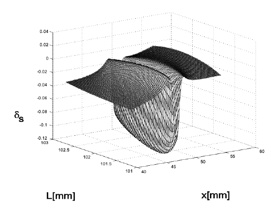
To gain insight into the sensitivity of a certain cavity configuration for KLM, it is interesting to compute the normalized beam size variations \(\delta_{s,t}\) as a function of the most critical cavity parameters. For the four-mirror cavity, the natural parameters to choose are the distance between the crystal and the pump mirror position, \(x\), and the mirror distance \(L\), see Figure 7.12. Figure 7.15 shows such a plot for the following cavity parameters \(R_1 = R_2 = 10\) cm, \(L_1 = 104\) cm, \(L_2 = 86\) cm, \(t = 2\) mm, \(n = 1.76\) and \(P = 200\) kW.
The Kerr lensing effect can be exploited in different ways to achieve mode locking.
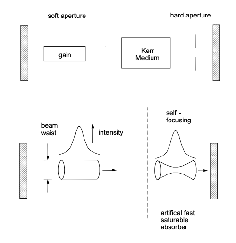
Soft-Aperture KLM
In the case of soft-aperture KLM, the cavity is tuned in such a way that the Kerr lensing effect leads to a shrinkage of the laser mode when mode-locked. The non-saturated gain in a laser depends on the overlap of the pump mode and the laser mode. From the rate equations for the radial photon distribution \(N(r)\) and the inversion \(N_P (r)\) of a laser, which are proportional to the intensities of the pump beam and the laser beam, we obtain a gain, that is proportional to the product of \(N(r)\) and \(N_P(r)\). If we assume that the focus of the laser mode and the pump mode are at the same position and neglect the variation of both beams as a function of distance, we obtain
\[\begin{array} {rcl} {g} & \sim & {N(r)*N_p(r) r dr} \\ {} & \sim & {\int_{0}^{\infty} \dfrac{2P_P}{\pi w_P^2} \exp \left [-\dfrac{2r^2}{w_P^2} \right ] \dfrac{2}{\pi w_L^2} \exp \left [-\dfrac{2r^2}{w_L^2} \right ] r dr} \end{array}\nonumber \]
With the beam cross sections of the pump and the laser beam in the gain medium, \(A_P = \pi w_P^2\) and \(A_L = \pi w_L^2\), we obtain
\[g \sim \dfrac{1}{A_p + A_L} \nonumber. \nonumber \]
If the pump beam is much stronger focused in the gain medium than the laser beam, a shrinkage of the laser mode cross section in the gain medium leads to an increased gain. When the laser operates in steady state, the change in saturated gain would have to be used for the investigation. However, the general argument carries through even for this case. Figure 7.16 shows the variation of the laser mode size in and close to the crystal in a soft-aperture KLM laser due to self-focusing.
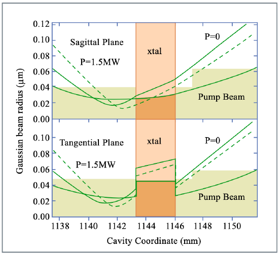
Figure by MIT OCW.
Hard-Aperture KLM
In a hard-aperture KLM-Laser, one of the resonator arms contains (usually close to the end mirrors) an aperture such that it cuts the beam slightly. When Kerr lensing occurs and leads to a shrinkage of the beam at this position, the losses of the beam are reduced. Note, that depending on whether the aperture is positioned in the long or short arm of the resontor, the operating point of the cavity at which Kerr lensing favours or opposes mode-locking may be quite different (see Figure 7.13).