
9.2: Noise in Mode-locked Lasers
- Page ID
- 44675

Within this framework the response of the laser to noise can be easily included. The spontaneous emission noise due to the amplifying medium with saturated gain gs and excess noise factor \(\Theta\) leads to additive white noise in the perturbed master equation (9.1.5) with \(L_{pert} = \xi (t, T)\), where \(\xi\) is a white Gaussian noise source with autocorrelation function
\[\langle \xi (t', T') \xi (t, T) \rangle = T_R^2 P_n \delta (t - t') \delta (T -T') \nonumber \]
where the spontaneous emission noise energy \(P_n \cdot T_R\) with
\[P_n = \Theta \dfrac{2g_s}{T_R} \hbar \omega_c = \Theta \dfrac{\hbar \omega_c}{\tau_p} \nonumber \]
is added to the pulse within each roundtrip in the laser. \(\tau_p\) is the cavity decay time or photon lifetime in the cavity. Note, that the noise is approximated by white noise, i.e. uncorrelated noise on both time scales \(t,T\). The noise between different round-trips is certainly uncorrelated. However, white noise on the fast time scale \(t\), assumes a flat gain, which is an approximation. By projecting out the equations of motion for the pulse parameters in the presence of this noise according to (9.1.7)-(9.1.12), we obtain the additional noise sources which are driving the energy, center frequency, timing and phase fluctuations in the mode-locked laser
\[\dfrac{\partial}{\partial T} \Delta w = -\dfrac{1}{\tau_w} \Delta w + S_w (T), \nonumber \]
\[\dfrac{\partial}{\partial T} \Delta \theta (T) = \dfrac{2\phi_o}{T_R} \dfrac{\Delta w}{w_o} \Delta w + S_{\theta} (T), \nonumber \]
\[\dfrac{\partial}{\partial T} \Delta p (T) = -\dfrac{1}{\tau_p} \Delta p + S_{p} (T), \nonumber \]
\[\dfrac{\partial}{\partial T} \Delta t= -\dfrac{2|D|}{T_R} \Delta p + S_{t} (T), \nonumber \]
with
\[S_w (T) = \dfrac{1}{T_R} \text{Re} \left \{\int_{-\infty}^{+\infty} \hat{f}_w^* (t) \xi (T, t) dt \right \}, \nonumber \]
\[S_{\theta} (T) = \dfrac{1}{T_R} \text{Re} \left \{\int_{-\infty}^{+\infty} \hat{f}_{\theta}^* (t) \xi (T, t) dt \right \}, \nonumber \]
\[S_p (T) = \dfrac{1}{T_R} \text{Re} \left \{\int_{-\infty}^{+\infty} \hat{f}_p^* (t) \xi (T, t) dt \right \}, \nonumber \]
\[S_t (T) = \dfrac{1}{T_R} \text{Re} \left \{\int_{-\infty}^{+\infty} \hat{f}_t^* (t) \xi (T, t) dt \right \}, \nonumber \]
The new reduced noise sources obey the correlation functions
\[\langle S_w (T') S_w (T) \rangle = \dfrac{P_n}{4\omega_0} \delta (T - T'), \nonumber \]
\[\langle S_{\theta} (T') S_{\theta} (T) \rangle = \dfrac{4}{3} \left (1 + \dfrac{\pi^2}{12} \right ) \dfrac{P_n}{w_o} \delta (T - T'), \nonumber \]
\[\langle S_p (T') S_p (T) \rangle = \dfrac{4}{3} \dfrac{P_n}{w_o} \delta (T - T'), \nonumber \]
\[\langle S_t (T') S_t (T) \rangle = \dfrac{\pi^2}{3} \dfrac{P_n}{w_o} \delta (T - T'), \nonumber \]
\[\langle S_i (T') S_j (T) \rangle = 0 \text{ for } i \ne j. \nonumber \]
The power spectra of amplitude, phase, frequency and timing fluctuations are defined via the Fourier transforms of the autocorrelation functions
\[|\Delta \hat{w} (\Omega)|^2 = \int_{-\infty}^{+\infty} \langle \Delta \hat{w} (T + \tau) \Delta \hat{w} (T) \rangle e^{-j\Omega \tau} d\tau , \text{ etc.} \nonumber \]
After a short calculation, the power spectra due to amplifier noise are
\[\left |\dfrac{\Delta \hat{w} (\Omega)}{w_o} \right |^2 = \dfrac{4}{1/\tau_w^2 + \Omega^2} \dfrac{P_n}{w_o},\label{eq9.2.17} \]
\[|\Delta \hat{\theta} (\Omega)|^2 = \dfrac{1}{\Omega^2} \left [\dfrac{4}{3} \left (1 + \dfrac{\pi^2}{12} \right ) \dfrac{P_n}{w_o} + \dfrac{16}{(1/\tau_p^2 + Omega^2)} \dfrac{\phi_o^2}{T_R^2} \dfrac{P_n}{w_o}\right ], \nonumber \]
\[\left |\Delta \hat{p} (\Omega) \tau \right |^2 = \dfrac{1}{1/\tau_p^2 + \Omega^2} \dfrac{4}{3} \dfrac{P_n}{w_o},\label{eq9.2.19} \]
\[\left | \dfrac{\Delta \hat{t} (\Omega)}{\tau} \right |^2 = \dfrac{1}{\Omega^2} \left [\dfrac{\pi^2}{3} \dfrac{P_n}{w_o} + \dfrac{1}{(1/\tau_{\omega}^2 + \Omega^2)} \dfrac{4}{3} \dfrac{4|D|^2}{T_R^2 \tau^4} \dfrac{P_n}{w_o} \right ]. \nonumber \]
These equations indicate, that energy and center frequency fluctuations become stationary with mean square fluctuations
\[\left \langle \left ( \dfrac{\Delta w}{w_o} \right )^2 \right \rangle = 2 \dfrac{P_n \tau_w}{w_o} \nonumber \]
\[\langle (\Delta \omega \tau )^2 \rangle = \dfrac{2}{3} \dfrac{P_n \tau_p^2}{w_o} \nonumber \]
whereas the phase and timing undergo a random walk with variances
\[\begin{array} {rcl} {\sigma_{\theta} (T)} & = & {\langle ( \Delta \theta (T) - \Delta \theta (0))^2 \rangle = \dfrac{4}{3} \left (1 + \dfrac{\pi^2}{12} \right ) \dfrac{P_n}{w_o} |T|} \\ {} & \ & {+16 \dfrac{\phi_o^2}{T_R^2} \dfrac{P_n}{w_o} \tau_p^3 \left (\exp \left [-\dfrac{|T|}{\tau_p} \right ] - 1 + \dfrac{|T|}{\tau_w} \right )} \end{array} \nonumber \]
\[\begin{array} {rcl} {\sigma_t (T)} & = & {\left \langle \left ( \dfrac{\Delta t(T) - \Delta t (0)}{\tau} \right )^2 \right \rangle = \dfrac{\pi^2}{3} \dfrac{P_n}{w_o} |T|} \\ {} & \ & {+ \dfrac{4}{3} \dfrac{4|D|^2}{T_R^2 \tau^4} \dfrac{P_n}{w_o} \tau_{\omega}^3 \left (\exp \left [-\dfrac{|T|}{\tau_p} \right ] - 1 + \dfrac{|T|}{\tau_p} \right )} \end{array} \nonumber \]
The phase noise causes the fundamental finite width of every line of the mode-locked comb in the optical domain. The timing jitter leads to a finite linewidth of the detected microwave signal, which is equivalent to the lasers fundamental fluctuations in repetition rate. In the strict sense, phase and timing in a free running mode-locked laser (or autonomous oscillator) are not anymore stationary processes. Nevertheless, since we know these are Gaussian distributed variables, we can compute the amplitude spectra of phasors undergoing phase diffusion processes rather easily. The phase difference \(\varphi = \Delta \theta (T) - \Delta \theta (0)\) is a Gaussian distributed variable with variance σ and propability distribution
\[p(\varphi) = \dfrac{1}{\sqrt{2\pi \sigma}} e^{-\tfrac{\varphi^2}{2\sigma}}, \text{ with } \sigma = \langle \varphi^2 \rangle. \nonumber \]
Therefore, the expectation value of a phasor with phase \(\phi\) is
\[\begin{array} {rcl} {\langle e^{j\varphi} \rangle} & = & {\dfrac{1}{\sqrt{2\pi \sigma}} \int_{-\infty}^{+\infty} e^{-\tfrac{\varphi^2}{2\sigma}} e^{j \varphi} d \varphi} \\ {} & = & {e^{-\tfrac{1}{2} \sigma}} \end{array}\label{eq9.2.26} \]
Optical Spectrum
\[a(t, T) = \left (A_0 \text{sech} (\dfrac{t - t_0}{\tau}) + a_c (T, t) \right ) e^{-j \phi_0 \tfrac{T}{T_R}} \nonumber \]
In the presence of noise the laser output changes from eq.(9.1) to a random process. Neglecting the background continuum we obtain:
\[\begin{array} {c} {A(t, T = m T_R) = \sum_{m = -\infty}^{+\infty} (A_0 + \Delta A(m T_R)) \text{sech } \left (\dfrac{t - mT_R - \Delta t (mT_R)}{\tau} \right ) } \\ {e^{j \Delta \phi_{CE} \cdot m} e^{j(\omega_c + \Delta p (mT_R)) t} e^{-j\Delta \theta (mT_R)}} \end{array}\label{eq9.2.28} \]
For simplicity, we will neglect in the following amplitude and carrier frequency fluctuations in Eq.(\(\ref{eq9.2.28}\)), because they are bounded and become only important at large offsets from the comb. However, we keep them in the expressions for the phase and timing jitter Eqs.(\(\ref{eq9.2.17}\)) and (\(\ref{eq9.2.19}\)). We assume a stationary process, so that the optical power spectrum can be computed from
\[S(\omega) = \lim_{T = 2NT_R \to \infty} \dfrac{1}{T} \langle \hat{A}_T^* (\omega) \hat{A}_T (\omega) \rangle\label{eq9.2.29} \]
with the spectra related to a finite time interval
\[\begin{array} {rcl} {\hat{A}_T (\omega) = \int_{-T}^T A(t) e^{-j \omega t} dt} & = & {\hat{a}_0 (\omega - \omega_c) \sum_{m = -N}^{N} e^{jmT_R (\tfrac{\Delta \phi_{CE}}{T_R} - \omega)}} \\ {} & \ & {e^{-j[(\omega - \omega_c)\Delta t (mT_R) + \Delta \theta (mT_R)]}} \end{array} \nonumber \]
where \(\hat{a}_0 (\omega)\) is the Fourier transform of the pulse shape. In this case
\[\hat{a}_0 (\omega) = \int_{-\infty}^{\infty} A_0 \text{sech} (\dfrac{t}{\tau}) e^{-j \omega t} dt = A_0 \pi \tau \text{sech} (\dfrac{\pi}{2} \omega \tau) \nonumber \]
With (\(\ref{eq9.2.29}\)) the optical spectrum of the laser is given by
\[\begin{array} {rcl} {S(\omega)} & = & {\lim_{N \to \infty} |\hat{a}_0 (\omega - \omega_c)|^2 \dfrac{1}{2NT_R} \sum_{m' = -N}^{N} \sum_{m = -N}^{M} e^{j T_R (\tfrac{\phi_{CE}}{T_R} - \omega)(m - m')}} \\ {} & \ & {\langle e^{+j [2\pi (f - f_c) (\Delta t (mT_R) - \Delta t (m'T_R)) - (\theta (m T_R) - \theta (m' T_R))]} \rangle} \end{array} \nonumber \]
Note, that the difference between the phases and the timing only depends on the difference \(k = m−m'\). In the current model phase and timing fluctuations are uncorrelated. Therefore, for \(N \to \infty\) we obtain
\[\begin{array} {rcl} {S(\omega)} & = & {|\hat{a}_0 (\omega - \omega_c)|^2 \tfrac{1}{T_R} \sum_{k' = -\infty}^{\infty} e^{jT_R (\tfrac{\Delta \phi_{CE}}{T_R} - \omega) k}} \\ {} & \ & {\langle e^{+j[2\pi (\omega - \omega_0)(\Delta t ((m + k) T_R) - \Delta t (m T_R))]} \rangle \langle e^{-j (\theta ((m + k) T_R) - \theta (m T_R))} \rangle} \end{array} \nonumber \]
The expectation values are exactly of the type calculated in (\(\ref{eq9.2.26}\)), which leads to
\[\begin{array} {rcl} {S(\omega)} & = & {\dfrac{|\hat{a}_0 (\omega - \omega_c)|^2}{T_R} \sum_{k' = -\infty}^{\infty} e^{jT_R (\tfrac{\phi_{CE}}{T_R} - \omega)k} e^{-\tfrac{1}{2} \sigma_{\theta} (kT_R)}} \\ {} & \ & {e^{-\tfrac{1}{2} [((\omega - \omega_c)\tau)^2 \sigma_t (kT_R)]}} \end{array}\label{eq9.2.34} \]
Most often we are interested in the noise very close to the lines at frequency offsets much smaller than the inverse energy and frequency relaxation times \(\tau_w\) and \(\tau_p\). This is determined by the long term behavior of the variances, which grow linearly in \(|T|\)
\[\sigma_{\theta} (T) = \dfrac{4}{3} \left (1 + \dfrac{\pi^2}{12} + 16 \dfrac{\tau_w^2}{T_R^2} \phi_o^2 \right ) \dfrac{P_n}{w_o} |T| = 2 \Delta \omega_{\phi} |T|, \nonumber \]
\[\sigma_t (T) = \dfrac{1}{3} \left (\pi^2 + \dfrac{\tau_p^2}{T_R^2} \left (\dfrac{D}{\tau^2} \right )^2 \right ) \dfrac{P_n}{w_o} |T| = 4 \Delta \omega_t |T|, \nonumber \]
with the rates
\[\Delta \omega_{\phi} = \dfrac{2}{3} \left (1 + \dfrac{\pi^2}{12} + 16 \dfrac{\tau_w^2}{T_R^2} \phi_o^2 \right ) \dfrac{P_n}{w_o},\label{eq9.2.37} \]
\[\Delta \omega_t = \dfrac{1}{6} \left (\pi^2 + \dfrac{\tau_p^2}{T_R^2} \left (\dfrac{D}{\tau^2} \right )^2 \right ) \dfrac{P_n}{w_o}.\label{eq9.2.38} \]
From the Poisson formula
\[\sum_{k = -\infty}^{+ \infty} h[k] e^{-j kx} = \sum_{n = -\infty}^{+\infty} G(x + 2n\pi) \nonumber \]
where
\[G(x) = \int_{-\infty}^{+\infty} h[k] e^{-jkx} dk, \nonumber \]
and Eqs.(\(\ref{eq9.2.34}\)) to (\(\ref{eq9.2.38}\)) we finally arrive at the optical line spectrum of the mode-locked laser
\[S(\omega) = \dfrac{|\hat{a}_0 (\omega - \omega_c)|^2}{T_R^2} \sum_{n = -\infty}^{+\infty} \dfrac{2\Delta \omega_n}{(\omega - \omega_n)^2 + \Delta \omega_n^2} \nonumber \]
which are Lorentzian lines at the mode comb positions.
\[\omega_n = \omega_c + n \omega_R - \dfrac{\Delta \phi_{CE}}{T_R}, \nonumber \]
\[= \dfrac{\Delta \phi_{CE}}{T_R} + n_R' \omega, \nonumber \]
with a half width at half maximum of
\[\Delta \omega_n = \Delta \omega_{\phi} + [\tau (\omega_n - \omega_c)]^2 \Delta \omega_t. \nonumber \]
Estimating the number of modes M included in the comb by
\[M = \dfrac{T_R}{\tau}, \nonumber \]
we see that the contribution of the timing fluctuations to the linewidth of the comb lines in the center of the comb is negligible. Thus the linewidth of the comb in the center is given by (\(\ref{eq9.2.37}\))
\[\Delta \omega_{\phi} = \dfrac{2}{3} \left (1 + \dfrac{\pi^2}{12} + 16 \dfrac{\tau_w^2}{T_R^2} \phi_o^2 \right ) \dfrac{\Theta 2 g_s}{N_0 T_R} \nonumber \]
\[\dfrac{2}{3} \left (1 + \dfrac{\pi^2}{12} + 16 \dfrac{\tau_w^2}{T_R^2} \phi_o^2 \right ) \dfrac{\Theta}{N_0 \tau_p} \nonumber \]
where \(N_0 = \tfrac{w_o}{\hbar \omega_c}\) is the number of photons in the cavity and \(\tau_p = T_R /(2l)\) is the photon lifetime in the cavity. Note that this result for the mode-locked laser is closely related to the Schawlow-Towns linewidth of a continuous wave laser which is \(\Delta f_{\phi} = \tfrac{\Theta}{2\pi N_0 \tau_p}\). For a solid-state laser at around \(1\mu m\) wavelength with a typical intracavity pulse energy of 50 nJ corresponding to \(N_0 = 2.5 \cdot 10^{11}\) photons and 100 MHz repetition rate with a 10% output coupler and an excess noise figure of \(\Theta = 2\), we obtain \(\Delta f_{\phi}^{\sim} \tfrac{\Theta}{3\pi N_0 \tau_p} = 8\mu Hz\) without the amplitude to phase conversion term depending on the nonlinear phase shift \(\phi_o\). These intrinsic linewidths are due to fluctuations happening on a time scale faster than the round-trip time and, therefore, can not be compensated by external servo control mechanisms. For sub-10 fs lasers, the spectra fill up the full gain bandwidth and the KLM is rather strong, so that the ampli- tude and center frequency relaxation times are on the order of 10-100 cavity roundtrips. In very short pulse Ti:sapphire lasers nonlinear phase shifts are on the order of 1 rad per roundtrip. Then most of the fluctuations are due to amplitude fluctuations converted into phase jitter. This contributions can increase the linewidth by a factor of 100-10000, which may bring the linewidth to the mHz and Hz level.
Microwave Spectrum
Not only the optical spectrum is of interest als the spectrum of the photo detected output of the laser is of intrest. Simple photo detection can convert the low jitter optical pulse stream into a comb of extremely low phase noise microwave signals. The photo detector current is proportional to the output power of the laser. From Eq.(\(\ref{eq9.2.28}\)) we find
\[\begin{array} {rcl} {I(t)} & = & {\eta \dfrac{e}{\hbar \omega_c} |A(T, t)|^3 = \eta \dfrac{e}{\hbar \omega_c \tau} \times } \\ {} & \ & {\sum_{m = -\infty}^{+\infty} (w_0 + \Delta w (mT_R)) \dfrac{1}{2} \text{sech}^2 \left (\dfrac{t - mT_R - \Delta t (mT_R)}{\tau} \right ),} \end{array} \nonumber \]
where \(\eta\) is the quantum efficiency. For simplicity we neglect again the amplitude noise and consider only the consequences due to the timing jitter. Then we obtain for the Fourier Transform of the photo current
\[\hat{I}_T (\omega) = \eta \dfrac{ew_0}{\hbar \omega_0 \tau} |a_0|^2 (\omega) \sum_{m =-N}^{+N} e^{-j \omega (mT_R + \Delta t (mT_R))}, \nonumber \]
\[|a_0|^2 (\omega) = \int_{-\infty}^{\infty} \dfrac{1}{2} \text{sech}^2 (x) e^{-\omega \tau x} dx \nonumber \]
\[= \dfrac{\pi \omega \tau}{\text{sinh} (\tfrac{\pi}{2} \omega \tau)}, \nonumber \]
and its power spectrum according to Eq.(\(\ref{eq9.2.29}\))
\[\begin{array} {rcl} {S_I (\omega)} & = & {\dfrac{(\eta e N_0)^2}{T_R} ||a_0|^2 (\omega)|^2 \sum_{k = -\infty}^{+ \infty} e^{-j \omega k T_R} \langle e^{-j\omega (\Delta t (k T_R) - \Delta t (0))} \rangle,} \\ {} & = & {\dfrac{(\eta e N_0)^2}{T_R} ||a_0|^2 (\omega)|^2 \sum_{k = -\infty}^{+ \infty} e^{-j \omega k T_R} e^{-\tfrac{1}{2}[(\omega \tau)^2 \sigma_t (kT_R)]}} \end{array} \nonumber \]
Using the Poisson formula again results in
\[\begin{array} {rcl} {S_I (\omega)} & = & {\dfrac{(\eta e N_0)^2}{T_R} ||a_0|^2 (\omega)|^2 \sum_{k = -\infty}^{+ \infty} e^{-j \omega k T_R} e^{-j\omega (\Delta t (k T_R) - \Delta t (0))},} \\ {} & = & {\dfrac{(\eta e N_0)^2}{T_R} ||a_0|^2 (\omega)|^2 \sum_{k = -\infty}^{+ \infty} \dfrac{2\Delta \omega_{I,n}}{(\omega - n \omega_R)^2 + \Delta \omega_{I,n}^2}} \end{array} \nonumber \]
with the linewidth \(\Delta \omega_{I,n}\) of the n-th harmonic
\[\begin{array} {rcl} {\Delta \omega_{I,n}} & = & {\left (2\pi n \dfrac{\tau}{T_R} \right )^2 \Delta \omega_t} \\ {} & = & {\left (\dfrac{2\pi n}{M} \right )^2 \Delta \omega_t} \end{array} \nonumber \]
The fundamental line \((n = 1)\) of the microwave spectrum has a width which is \(M^2\)−times smaller than the optical linewidth. For a 10-fs laser with 100 MHz repetition rate, the number of modes \(M\) is about a million.
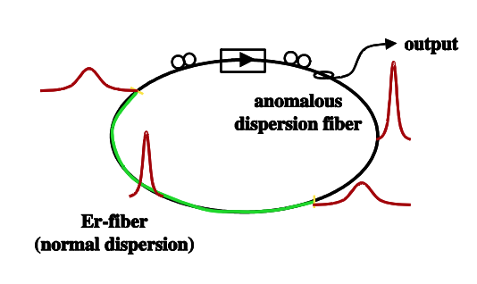
Example: Yb-fiber laser
Figure 9.3 shows the schematic of a stretched pulse modelocked laser operating close to zero dispersion. Therefore, the contribution of the Gordon-Haus jitter should be minimized. In fact, it has been shown and discussed that these types of lasers reach minimum jitter levels [2][3][4].
The timing jitter of the stretched pulse laser shown in Figure is computed in table 9.1.
The theoretical results above are derived with soliton perturbation theory. The stretched pulse modelocked laser in Figure 9.3 is actually far from being a soliton laser, see [3][4]. The pulse is breathing considerably during
| Gain Half-Width Half Maximum | \(\Omega_g = 2\pi \cdot \tfrac{0.3 \mu m/fs}{(1 \mu m)^2} 0.02 \mu m = 38 THz\) |
| Saturated gain | \(g_s = 1.2\) |
| Pulse width | \(\tau_{FWHM} = 50fs, \tau = \tau_{FWHM}/1.76 = 30fs\) |
| Pulse repetition time | \(T_R = 12 ns\) |
| Decay time for center freq. fluctuations | \(\tfrac{1}{\tau_p} = \tfrac{4}{3} \tfrac{g_s}{\Omega_g^2 \tau^2 T_R} = \tfrac{4}{3} \tfrac{1}{T_R}\) |
| Intracavity power | \(P = 100 mW\) |
| Intra cavity pulse energy /photon number | \(w_o = 1.2nJ, N_0 = 0.6 \cdot 10^{10}\) |
| Noise power spectral density | \(P_n = \Theta \tfrac{2g_s}{T_R} \hbar w_o\) |
| Amplifier excess noise factor | \(\Theta = 10\) |
| ASE noise | \(\tfrac{P_n}{w_o} = \Theta \tfrac{2g_s}{T_R N_0} = \tfrac{1}{3} Hz\) |
| Dispersion | \(5000 fs^2\) |
| Frequency-to-timing conv. | \(\tfrac{4}{\pi^2} \tfrac{4|D|^2}{\tau^4} \tfrac{\tau_p^2}{T_R^2} = (\tfrac{2}{\pi} \tfrac{3}{4} \tfrac{3 \cdot 10000}{1000})^2 = (3.7)^2\) |
| Timing jitter density | \(|\tfrac{\Delta \hat{t} (\Omega)}{\tau}|^2 = \tfrac{1}{\Omega^2} \tfrac{\pi^2}{3} \tfrac{P_n}{w_o} (1 + \tfrac{4}{\pi^2} \tfrac{4|D|^2}{\tau^4} \tfrac{1}{(T_R^2/\tau_p^2 + T_R^2 \Omega^2)})\) |
| Timing jitter \([f_{\min},f_{\max}]\) for \(f_{\min} << 1/\tau_p\), \(f_{\min} = 10kHz\), \(D = 5000 fs^2\) | \(\Delta t = \tau \sqrt{\tfrac{1}{12 \cdot f_{\min}} \tfrac{P_n}{w_o} (1 + \tfrac{4}{\pi^2} \tfrac{4|D|^2}{\tau^4} \tfrac{\tau_p^2}{T_R^2})} = 0.2 fs\) |
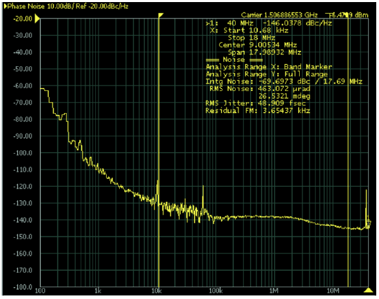
passage through the cavity up to a factor of 10. Therefore, the theory should take that into account by assuming an average pulse width when the noise is added in the cavity. For more details see [3][4]. In reality, these quantum limited (ASE) and rather small optical and microwave linewidths are difficult to observe, because they are most often swamped by technical noise such as fluctuations in pump power, which may case gain fluctuations, or mirror vibrations, air-density fluctuations or thermal drifts, which directly cause changes in the lasers repetition rate. Figure 9.4 shows the single-sideband phase noise spectrum \(L(f)\) of the N=32nd harmonic of the fundamental repetition rate, i.e 1.3 GHz, in the photo current spectrum 9.70. The phase of the N=32nd harmonic of the photocurrent 9.65 is directly related to the timing jitter by
\[\Delta \phi (T) = 2\pi Nf_R \Delta t (T) \nonumber \]
The single-sideband phase noise is the power spectral density of these phase fluctuations defined in the same way as the power spectral density of the photocurrent itself, i.e.
\[L(f) = 2\pi S_{\Delta \phi} (\omega) \nonumber \]
The phase fluctuations in a certain frequency intervall can then be easily evaluated by
\[\Delta \phi^2 = 2\int_{f_{\min}}^{f_{\max}} L(f) df. \nonumber \]
And the timing jitter is then
\[\Delta t = \dfrac{1}{2\pi Nf_R} \sqrt{2 \int_{f_{\min}}^{f_{\max}} L(f) df} \nonumber \]
For the measurements shown in Figure 9.4 we obtain for the integrated timing jitter from 10kHz to 20 MHz of 50 fs. This is about 200 times larger than the limits derived in table 9.1. This discrepancy comes from several effects, most notable amplitude to phase conversion in the photodetector during photodetection, an effect not yet well understood as well as other noise sources we might not have modelled, such as noise from the pump laser. However, these noise sources can be eliminated in principle by careful design and feed-back loops. Therefore, it is important to understand the dependence of the group and phase velocity on the intracavity power or pulse energy at least within the current basic model. Additional linear and nonlinear effects due to higher order linear dispersion or nonlinearities may cause additional changes in group and phase velocity, which might also create unusual dependencies of group and phase velocity on intracavity pulse energy. Here we discuss as an example the impact of the instantaneous Kerr effect on group and phase velocity of a soliton like pulse.