
9.1: The Mode Comb
- Page ID
- 44674
\( \newcommand{\vecs}[1]{\overset { \scriptstyle \rightharpoonup} {\mathbf{#1}} } \)
\( \newcommand{\vecd}[1]{\overset{-\!-\!\rightharpoonup}{\vphantom{a}\smash {#1}}} \)
\( \newcommand{\dsum}{\displaystyle\sum\limits} \)
\( \newcommand{\dint}{\displaystyle\int\limits} \)
\( \newcommand{\dlim}{\displaystyle\lim\limits} \)
\( \newcommand{\id}{\mathrm{id}}\) \( \newcommand{\Span}{\mathrm{span}}\)
( \newcommand{\kernel}{\mathrm{null}\,}\) \( \newcommand{\range}{\mathrm{range}\,}\)
\( \newcommand{\RealPart}{\mathrm{Re}}\) \( \newcommand{\ImaginaryPart}{\mathrm{Im}}\)
\( \newcommand{\Argument}{\mathrm{Arg}}\) \( \newcommand{\norm}[1]{\| #1 \|}\)
\( \newcommand{\inner}[2]{\langle #1, #2 \rangle}\)
\( \newcommand{\Span}{\mathrm{span}}\)
\( \newcommand{\id}{\mathrm{id}}\)
\( \newcommand{\Span}{\mathrm{span}}\)
\( \newcommand{\kernel}{\mathrm{null}\,}\)
\( \newcommand{\range}{\mathrm{range}\,}\)
\( \newcommand{\RealPart}{\mathrm{Re}}\)
\( \newcommand{\ImaginaryPart}{\mathrm{Im}}\)
\( \newcommand{\Argument}{\mathrm{Arg}}\)
\( \newcommand{\norm}[1]{\| #1 \|}\)
\( \newcommand{\inner}[2]{\langle #1, #2 \rangle}\)
\( \newcommand{\Span}{\mathrm{span}}\) \( \newcommand{\AA}{\unicode[.8,0]{x212B}}\)
\( \newcommand{\vectorA}[1]{\vec{#1}} % arrow\)
\( \newcommand{\vectorAt}[1]{\vec{\text{#1}}} % arrow\)
\( \newcommand{\vectorB}[1]{\overset { \scriptstyle \rightharpoonup} {\mathbf{#1}} } \)
\( \newcommand{\vectorC}[1]{\textbf{#1}} \)
\( \newcommand{\vectorD}[1]{\overrightarrow{#1}} \)
\( \newcommand{\vectorDt}[1]{\overrightarrow{\text{#1}}} \)
\( \newcommand{\vectE}[1]{\overset{-\!-\!\rightharpoonup}{\vphantom{a}\smash{\mathbf {#1}}}} \)
\( \newcommand{\vecs}[1]{\overset { \scriptstyle \rightharpoonup} {\mathbf{#1}} } \)
\(\newcommand{\longvect}{\overrightarrow}\)
\( \newcommand{\vecd}[1]{\overset{-\!-\!\rightharpoonup}{\vphantom{a}\smash {#1}}} \)
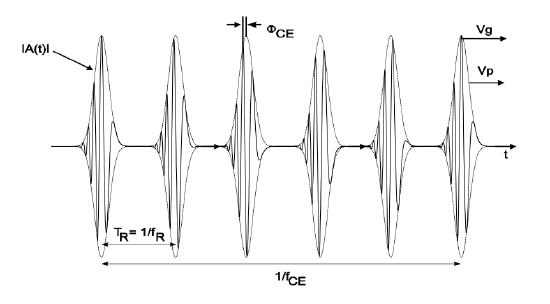
\(\newcommand{\avec}{\mathbf a}\) \(\newcommand{\bvec}{\mathbf b}\) \(\newcommand{\cvec}{\mathbf c}\) \(\newcommand{\dvec}{\mathbf d}\) \(\newcommand{\dtil}{\widetilde{\mathbf d}}\) \(\newcommand{\evec}{\mathbf e}\) \(\newcommand{\fvec}{\mathbf f}\) \(\newcommand{\nvec}{\mathbf n}\) \(\newcommand{\pvec}{\mathbf p}\) \(\newcommand{\qvec}{\mathbf q}\) \(\newcommand{\svec}{\mathbf s}\) \(\newcommand{\tvec}{\mathbf t}\) \(\newcommand{\uvec}{\mathbf u}\) \(\newcommand{\vvec}{\mathbf v}\) \(\newcommand{\wvec}{\mathbf w}\) \(\newcommand{\xvec}{\mathbf x}\) \(\newcommand{\yvec}{\mathbf y}\) \(\newcommand{\zvec}{\mathbf z}\) \(\newcommand{\rvec}{\mathbf r}\) \(\newcommand{\mvec}{\mathbf m}\) \(\newcommand{\zerovec}{\mathbf 0}\) \(\newcommand{\onevec}{\mathbf 1}\) \(\newcommand{\real}{\mathbb R}\) \(\newcommand{\twovec}[2]{\left[\begin{array}{r}#1 \\ #2 \end{array}\right]}\) \(\newcommand{\ctwovec}[2]{\left[\begin{array}{c}#1 \\ #2 \end{array}\right]}\) \(\newcommand{\threevec}[3]{\left[\begin{array}{r}#1 \\ #2 \\ #3 \end{array}\right]}\) \(\newcommand{\cthreevec}[3]{\left[\begin{array}{c}#1 \\ #2 \\ #3 \end{array}\right]}\) \(\newcommand{\fourvec}[4]{\left[\begin{array}{r}#1 \\ #2 \\ #3 \\ #4 \end{array}\right]}\) \(\newcommand{\cfourvec}[4]{\left[\begin{array}{c}#1 \\ #2 \\ #3 \\ #4 \end{array}\right]}\) \(\newcommand{\fivevec}[5]{\left[\begin{array}{r}#1 \\ #2 \\ #3 \\ #4 \\ #5 \\ \end{array}\right]}\) \(\newcommand{\cfivevec}[5]{\left[\begin{array}{c}#1 \\ #2 \\ #3 \\ #4 \\ #5 \\ \end{array}\right]}\) \(\newcommand{\mattwo}[4]{\left[\begin{array}{rr}#1 \amp #2 \\ #3 \amp #4 \\ \end{array}\right]}\) \(\newcommand{\laspan}[1]{\text{Span}\{#1\}}\) \(\newcommand{\bcal}{\cal B}\) \(\newcommand{\ccal}{\cal C}\) \(\newcommand{\scal}{\cal S}\) \(\newcommand{\wcal}{\cal W}\) \(\newcommand{\ecal}{\cal E}\) \(\newcommand{\coords}[2]{\left\{#1\right\}_{#2}}\) \(\newcommand{\gray}[1]{\color{gray}{#1}}\) \(\newcommand{\lgray}[1]{\color{lightgray}{#1}}\) \(\newcommand{\rank}{\operatorname{rank}}\) \(\newcommand{\row}{\text{Row}}\) \(\newcommand{\col}{\text{Col}}\) \(\renewcommand{\row}{\text{Row}}\) \(\newcommand{\nul}{\text{Nul}}\) \(\newcommand{\var}{\text{Var}}\) \(\newcommand{\corr}{\text{corr}}\) \(\newcommand{\len}[1]{\left|#1\right|}\) \(\newcommand{\bbar}{\overline{\bvec}}\) \(\newcommand{\bhat}{\widehat{\bvec}}\) \(\newcommand{\bperp}{\bvec^\perp}\) \(\newcommand{\xhat}{\widehat{\xvec}}\) \(\newcommand{\vhat}{\widehat{\vvec}}\) \(\newcommand{\uhat}{\widehat{\uvec}}\) \(\newcommand{\what}{\widehat{\wvec}}\) \(\newcommand{\Sighat}{\widehat{\Sigma}}\) \(\newcommand{\lt}{<}\) \(\newcommand{\gt}{>}\) \(\newcommand{\amp}{&}\) \(\definecolor{fillinmathshade}{gray}{0.9}\)Lets suppose the pulse envelope, repetition rate, and center frequency do not change any more. Then the corresponding time domain signal is sketched in Figure 9.1.
The pulse \(a(T = mT_r, t)\) is the steady state solution of the master equation describing the laser system, as studied in chapter 6. Let’s assume that the steady state solution is a purturbed soliton according to equation (6.3.3).
\[a(t, T) = \left (A_0 \text{sech} (\dfrac{t- t_0}{\tau}) + a_c (T, t) \right ) e^{-j \phi_0 \tfrac{T}{T_R}} \nonumber \]
with the soliton phase shift
\[\phi_0 = \dfrac{1}{2} \delta A_0^2 = \dfrac{|D|}{\tau^2} \nonumber \]
Thus, there is a carrier envelope phase shift \(\Delta \phi_{CE}\) from pulse to pulse given by
\[\begin{array} {rcl} {\Delta \phi_{CE}} & = & {\left (\dfrac{1}{v_g} - \dfrac{1}{v_p} \right )|_{\omega_c} 2L - \phi_0 + \text{mod}(2\pi)} \\ {} & = & {\omega_c T_R \left (1 - \dfrac{v_g}{v_p} \right ) - \phi_0 + \text{mod} (2\pi)} \end{array} \nonumber \]
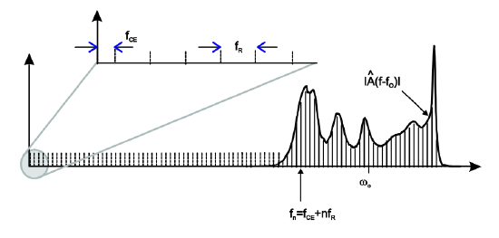
The Fourier transform of the unperturbed pulse train is
\[\begin{array} {rcl} {\hat{A} (\omega)} & = & {\hat{a} (\omega - \omega_c) \sum_{m = -\infty}^{+\infty} e^{j(\Delta \phi_{CE} - (\omega - \omega_c)T_R)m}} \\ {} & = & {\hat{a} (\omega - \omega_c) \sum_{m = -\infty}^{+\infty} e^{jmT_R (\tfrac{\Delta \phi_{CE}}{T_R} - \omega)}} \\ {} & = & {\hat{a} (\omega - \omega_c) \sum_{m = -\infty}^{+\infty} T_R \delta \left (\omega - \left (\dfrac{\Delta \phi_{CE}}{T_R} + n \omega_R \right ) \right )} \end{array} \nonumber \]
which is shown in Figure 9.2. Each comb line is shifted by the carrier-envelope offset frequency \(f_{CE} = \tfrac{\Delta \phi_{CE}}{2\pi T_R}\) from the origin
To obtain self-consistent equations for the repetition rate, center frequency and the other pulse parameters we employ soliton-perturbation theory. This is justified for the case, where the steady state pulse is close to a soliton, i.e. for the fast saturable absorber case, this is the chirp free solution, occuring when the ratio of gain filtering to dispersion is equal to the ratio of SAM action to self-phase modulation, see Equation (6.2.43). Then the pulse solution in the \(m\)−th roundtrip is a solution of the nonlinear Schrödinger Equation stabilized by the irreversible dynamics and subject to additional perturbations
\[T_R \dfrac{\partial}{\partial T} A = j D \dfrac{\partial^2}{\partial t^2} A - j \delta |A|^2 A + (g - l)A + D_f \dfrac{\partial^2}{\partial t^2} A + \gamma |A|^2 A + L_{pert}\label{eq9.1.5} \]
Due to the irreversible processes and the perturbations the solution to (\(\ref{eq9.1.5}\)) is a soliton like pulse with perturbations in amplitude, phase, frequency and timing plus some continuum
\[A(t, T) = [(A_o + \Delta A_o) \text{sech} [(t - \Delta t)/\tau] + a_c (T, t)] e^{-j\phi_o T/T_R} e^{j \Delta p (T) t} e^{-j \theta_0} \nonumber \]
with pulse energy \(w_0 = 2A_o^2 \tau\).
The perturbations cause fluctuations in amplitude, phase, center frequency and timing of the soliton and generate background radiation, i.e. continuum
\[\Delta A (T, t) = \Delta w(T) f_w (t) + \Delta \theta (T) f_{\theta} (t) + \Delta p(T) f_p (t) + \Delta t(T) f_t (t) + a_c (T, t). \nonumber \]
where, we rewrote the amplitude perturbation as an energy perturbation. The dynamics of the pulse parameters due to the perturbed Nonlinear Schrödinger Equation (\(\ref{eq9.1.5}\)) can be projected out from the perturbation using the adjoint basis and the orthogonality relation, see Chapter 3.5. Note, that the fi correspond to the first component of the vector in Eqs.(3.5.9) - (3.5.12). The dynamics of the pulse parameters due to the perturbed Nonlinear Schrödinger Equation (\(\ref{eq9.1.5}\)) can be projected out from the perturbation using the adjoint basis \(\hat{f}_i^*\) corresponding to the first component of the vector in Eqs.(3.5.31) - (3.5.34) and the new orthogonality relation
\[\text{Re} \left \{\int_{-\infty}^{+\infty} \hat{f}_i^* (t) f_j (t) dt \right \} = \delta_{i,j}. \nonumber \]
We obtain
\[\dfrac{\partial}{\partial T} \Delta w = -\dfrac{1}{\tau_w} \Delta w + \dfrac{1}{T_R} \text{Re} \left \{\int_{-\infty}^{+\infty} \hat{f}_w^* (t) L_{pert} (T, t) dt \right \} \nonumber \]
\[\dfrac{\partial}{\partial T} \Delta \theta (T) = \dfrac{2\phi_o}{T_R} \dfrac{\Delta w}{w_o} + \dfrac{1}{T_R} \text{Re} \left \{\int_{-\infty}^{+\infty} \hat{f}_{\theta}^* (t) L_{pert} (T, t) dt \right \} \nonumber \]
\[\dfrac{\partial}{\partial T} \Delta p(T) = -\dfrac{1}{\tau_p} \Delta p + \dfrac{1}{T_R} \text{Re} \left \{\int_{-\infty}^{+\infty} \hat{f}_p^* (t) L_{pert} (T, t) dt \right \} \nonumber \]
\[\dfrac{\partial}{\partial T} \Delta t = \dfrac{-2|D|}{T_R} \Delta \omega + \dfrac{1}{T_R} \text{Re} \left \{\int_{-\infty}^{+\infty} \hat{f}_t^* (t) L_{pert} (T, t) dt \right \} \nonumber \]
Note, that the irreversible dynamics does couple back the generated continuum to the soliton parameters. Here, we assume that this coupling is small and neglect it in the following, see [1]. Due to gain saturation and the parabolic filter pulse energy and center frequency fluctuations are damped with normalized decay constants
\[\dfrac{1}{\tau_w} = (2g_d - 2\gamma A_o^2) \nonumber \]
\[\dfrac{1}{\tau_p} = \dfrac{4}{3} \dfrac{g_s}{\Omega_g^2 \tau^2} \dfrac{1}{T_R} \nonumber \]
Here, \(g_s\) is the saturated gain and \(g_d\) is related to the differential gain by
\[g_s = \dfrac{g_o}{1 + \tfrac{w_o}{P_L T_R}} \nonumber \]
\[g_d = \dfrac{dg_s}{dw_o} \cdot w_o \nonumber \]
Note, in this model we assumed that the gain instantaneously follows the intracavity average power or pulse energy, which is not true in general. However, it is straight forward to include the relaxation of the gain by adding a dynamical gain model to the perturbation equations. For simplicity we shall neglect this here. Since the system is autonomous, there is no retiming and rephasing in the free running system.