
6.2: Fast Saturable Absorber Mode Locking
- Page ID
- 44662

The dynamics of a laser modelocked with a fast saturable absorber is again covered by the master equation (5.1.21) [3]. Now, the losses \(q\) react instantly on the intensity or power \(P(t) = |A(t)|^2\) of the field
\[q(A) = \dfrac{q_0}{1 + \tfrac{|A|^2}{P_A}},\label{eq6.2.1} \]
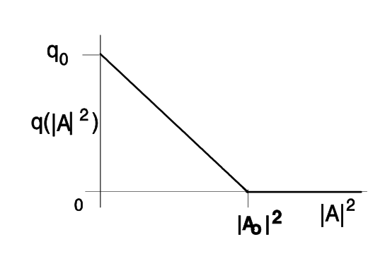
where \(P_A\) is the saturation power of the absorber. There is no analytic solution of the master equation (5.1.21) with the absorber response (\(\ref{eq6.2.1}\)). Therefore, we make expansions on the absorber response to get analytic insight. If the absorber is not saturated, we can expand the response (\(\ref{eq6.2.1}\)) for small intensities
\[q(A) = q_0 - \gamma |A|^2,\label{eq6.2.2} \]
with the saturable absorber modulation coefficient \(\gamma = q_0/P_A\). The constant nonsaturated loss \(q_0\) can be absorbed in the losses \(l_0 = l + q_0\). The resulting master equation is, see also Figure 6.3
\[T_R \dfrac{\partial A(T, t)}{\partial T} = \left [g - l_0 + D_f \dfrac{\partial^2}{\partial t^2} + \gamma |A|^2 + j D_2 \dfrac{\partial^2}{\partial t^2} - j \delta |A|^2 \right ] A(T, t).\label{eq6.2.3} \]
Image removed due to copyright restrictions. Please see:Keller, U., Ultrafast Laser Physics, Institute of Quantum Electronics, Swiss Federal Institute of Technology, ETH Hönggerberg—HPT, CH-8093 Zurich, Switzerland.
Figure 6.3: Schematic representation of the master equation for a passively modelocked laser with a fast saturable absorber.
Equation (\(\ref{eq6.2.3}\)) is a generalized Ginzburg-Landau equation well known from superconductivity with a rather complex solution manifold.
Without GDD and SPM
We consider first the situation without SPM and GDD, i.e. \(D_2 = \delta =0\)
\[T_R \dfrac{\partial A(T, t)}{\partial T} = \left [g - l_0 + D_f \dfrac{\partial ^2}{\partial t^2} + \gamma |A|^2 \right ] A (T, t).\label{eq6.2.4} \]
Up to the imaginary unit, this equation is still very similar to the NSE. To find the final pulse shape and width, we look for the stationary solution
\[T_R \dfrac{\partial A_s (T, t)}{\partial T} = 0.\label{eq6.2.5} \]
Since the equation is similar to the NSE, we try the following ansatz
\[A_s (T, t) = A_s (t) = A_0 \text{sech} \left (\dfrac{t}{\tau} \right ). \nonumber \]
Note, there is
\[\dfrac{d}{dx} \text{sech} x = - \text{tanh} x\ \text{sech} x, \nonumber \]
\[\begin{array} {rcl} {\dfrac{d^2}{dx^2} \text{sech} x} & = & {\text{tanh}^2 x\ \text{sech} x - \text{sech}^3 x,} \\ {} & = & {(\text{sech} x - 2 \text{sech}^3 x).} \end{array} \nonumber \]
Substitution of ansatz (\(\ref{eq6.2.5}\)) into the master equation (\(\ref{eq6.2.4}\)), assuming steady state, results in
\[0 = \left [(g - l_0) + \dfrac{D_f}{\tau^2} \left [1 - 2 \text{sech}^2 \left (\dfrac{t}{\tau} \right ) \right ] + \gamma |A_0|^2 \text{sech}^2 \left (\dfrac{t}{\tau} \right ) \right ] \cdot A_0 \text{sech} \left (\dfrac{t}{\tau} \right ). \nonumber \]
Comparison of the coefficients with the \(\text{sech}\)- and \(\text{sech}^3\)-expressions results in the conditions for the pulse peak intensity and pulse width \(\tau\) and for the saturated gain
\[\dfrac{D_f}{\tau^2} = \dfrac{1}{2} \gamma |A_0|^2,\label{eq6.2.10} \]
\[g = l_0 - \dfrac{D_f}{\tau^2}\label{eq6.2.11} \]
From Eq.(\(\ref{eq6.2.10}\)) and with the pulse energy of a sech pulse, see Eq.(3.3.6), \(W = 2|A_0|^2 \tau\),
\[\tau = \dfrac{4D_f}{\gamma W}.\label{eq6.2.12} \]
Equation (\(\ref{eq6.2.12}\)) is rather similar to the soliton width with the exception that the conservative pulse shaping effects GDD and SPM are replaced by gain dispersion and saturable absorption. The soliton phase shift per roundtrip is replaced by the difference between the saturated gain and loss in Equation (\(\ref{eq6.2.12}\)). It is interesting to have a closer look on how the difference between gain and loss \(\tfrac{D_f}{\tau^2}\) per round-trip comes about. From the master equation (\(\ref{eq6.2.4}\)) we can derive an equation of motion for the pulse energy according to
\[T_R \dfrac{\partial W(T)}{\partial T} = T_R \dfrac{\partial}{\partial T} \int_{-\infty}^{\infty} |A(T, t)|^2 \ dt \nonumber \]
\[= T_R \int_{-\infty}^{\infty} \left [A(T, t) * \dfrac{\partial}{\partial T} A(T, t) + c.c. \right ] \ dt\label{eq6.2.14} \]
\[= 2G (g_s, W) W, \nonumber \]
where \(G\) is the net energy gain per roundtrip, which vanishes when steady state is reached [3]. Substitution of the master equation into (\(\ref{eq6.2.14}\)) with
\[\int_{-\infty}^{\infty} (\text{sech}^2 x) dx = 2, \nonumber \]
\[\int_{-\infty}^{\infty} (\text{sech}^4 x) dx = \dfrac{4}{3}, \nonumber \]
\[-\int_{-\infty}^{\infty} \dfrac{d^2}{dx^2} (\text{sech} x) dx = \int_{-\infty}^{\infty} \left (\dfrac{d}{dx} \text{sech} x \right )^2 dx = \dfrac{2}{3}. \nonumber \]
results in
\[G(g_s, W) = g_s - l_0 - \dfrac{D_f}{3\tau^2} + \dfrac{2}{3} \gamma |A_0|^2\label{eq6.2.19} \]
\[ = g_s - l_0 + \dfrac{1}{2} \gamma |A_0|^2 = g_s - l_0 + \dfrac{D_f}{\tau^2} = 0\label{eq6.2.20} \]
with the saturated gain
\[g_s (W) = \dfrac{g_0}{1 + \tfrac{W}{P_L T_R}} \nonumber \]
Equation (\(\ref{eq6.2.20}\)) together with (\(\ref{eq6.2.12}\)) determines the pulse energy
\[\begin{array} {rcl} {g_s(W)} & = & {\dfrac{g_0}{1 + \tfrac{W}{P_L T_R} = l_0 - \dfrac{D_f}{\tau^2}} \\ {} & = & {l_0 - \dfrac{(\gamma W)^2}{16D_g}} \end{array} \nonumber \]
Figure 6.4 shows the time dependent variation of gain and loss in a laser modelocked with a fast saturable absorber on a normalized time scale Here, we assumed that the absorber saturates linearly with intensity up to a maximum value \(q_0 = \gamma A_0^2\). If this maximum saturable absorption is completely exploited see Figure 6.5.The minimum pulse width achievable with a given saturable absorption \(q0\) results from Eq.(\(\ref{eq6.2.10}\))
\[\dfrac{D_f}{\tau^2} = \dfrac{q_0}{2}, \nonumber \]
to be
\[\tau = \sqrt{\dfrac{2}{q_0}} \dfrac{1}{\Omega_f}.\label{6.2.24} \]
Image removed due to copyright restrictions. Please see: Kartner, F. X., and U. Keller. "Stabilization of soliton-like pulses with a slow saturable absorber." Optics Letters 20 (1990): 16-19.
Figure 6.4: Gain and loss in a passively modelocked laser using a fast saturable absorber on a normalized time scale \(x = t/\tau\). The absorber is assumed to saturate linearly with intensity according to \(q(A) = q_0 (1 - \tfrac{|A|^2}{A_0^2})\).
Note that in contrast to active modelocking, now the achievable pulse width is scaling with the inverse gain bandwidth, which gives much shorter pulses. Figure 6.4 can be interpreted as follows: In steady state, the saturated gain is below loss, by about one half of the exploited saturable loss before and after the pulse. This means, that there is net loss outside the pulse, which keeps the pulse stable against growth of instabilities at the leading and trailing edge of the pulse. If there is stable mode-locked operation, there must be always net loss far away from the pulse, otherwise, a continuous wave signal running at the peak of the gain would experience more gain than the pulse and would break through. From Eq.(\(\ref{eq6.2.19}\)) follows, that one third of the exploited saturable loss is used up during saturation of the aborber and actually only one sixth is used to overcome the filter losses due to the finite gain bandwidth. Note, there is a limit to the mimium pulse width, which comes about, because the saturated gain (\(\ref{eq6.2.11}\)) is \(g_s = l + \dfrac{1}{2} q_0\) and, therefore, from Eq.(\(\ref{eq6.2.24}\)), if we assume that the finite bandwidth of the laser is set by the gain, i.e. \(D_f = D_g = \dfrac{g}{\Omega_g^2}\) we obtain for \(q_0 \gg 1\)
\[\tau_{\min} = \dfrac{1}{\Omega_g} \nonumber \]
for the linearly saturating absorber model. This corresponds to mode locking over the full bandwidth of the gain medium, since for a sech-shaped pulse, the time-bandwidth product is 0.315, and therefore,
\[\Delta f_{FWHM} = \dfrac{0.315}{1.76 \cdot \tau_{\min}} = \dfrac{\Omega_g}{1.76 \cdot \pi}. \nonumber \]
As an example, for Ti:sapphire this corresponds to \(\Omega_g = 270\ THz\), \(\tau_{\min} 3.7\ fs\), \(\tau_{FWHM} = 6.5 \ fs\).
With GDD and SPM
After understanding what happens without GDD and SPM, we look at the solutions of the full master equation (\(\ref{eq6.2.3}\)) with GDD and SPM. It turns out, that there exist steady state solutions, which are chirped hyperbolic secant functions [4]
\[A_s(T, t) = A_0 \left ( \text{sech} \left ( \dfrac{t}{\tau} \right ) \right )^{1 + j \beta} e^{j\psi T/T_R},\label{eq6.2.26} \]
\[= A_0 \text{sech} \left (\dfrac{t}{\tau}\right ) \exp \left [j\beta \ln \text{sech} \left (\dfrac{t}{\tau}\right ) + j \psi T/T_R \right ]. \nonumber \]
Where \(\psi\) is the round-trip phase shift of the pulse, which we have to allow for. Only the intensity of the pulse becomes stationary. There is still a phase-shift per round-trip due to the difference between the group and phase velocity (these effects have been already transformed away) and the nonlinear effects. As in the last section, we can substitute this ansatz into the master equation and compare coefficients. Using the following relations
\[\dfrac{d}{dx} (f(x)^b) = bf(x)^{b-1} \dfrac{d}{dx} f(x) \nonumber \]
\[\dfrac{d}{dx} (\text{sech} x)^{(1 +j\beta)} = -(1 + j\beta) \text{tanh} x (\text{sech} x)^{(1 +j\beta)}, \nonumber \]
\[\dfrac{d^2}{dx^2} (\text{sech} x)^{(1 +j\beta)} = ((1 + j \beta)^2 - (2 + 3j\beta - \beta^2) \text{sech}^2 x) (\text{sech} x)^{(1 +j\beta)} \nonumber \]
in the master equation and comparing the coefficients to the same functions leads to two complex equations
\[\dfrac{1}{r^2} (D_f + j D_2)(2+3j\beta - \beta^2) = (\gamma - j \delta)|A_0|^2,\label{eq6.2.31} \]
\[l_0 - \dfrac{(1 + j\beta)^2}{\tau^2} (D_f + j D_2) = g - j \psi.\label{eq6.2.32} \]
These equations are extensions to Eqs.(\(\ref{eq6.2.11}\)) and (\(\ref{eq6.2.12}\)) and are equivalent to four real equations for the phase-shift per round-trip \(\psi\), the pulse width \(\tau\), the chirp \(\beta\) and the peak power \(|A_0|^2\) or pulse energy. The imaginary part of Eq.(\(\ref{eq6.2.32}\)) determines the phase-shift only, which is most often not of importance. The real part of Eq.(\(\ref{eq6.2.32}\)) gives the saturated gain
\[g = l_0 - \dfrac{1 - \beta^2}{\tau^2} D_f + \dfrac{2\beta D_2}{\tau^2}.\label{eq6.2.33} \]
The real part and imaginary part of Eq.(\(\ref{eq6.2.31}\)) give
\[\dfrac{1}{\tau^2} [D_f (2 - \beta^2) - 3\beta D_2] = \gamma |A_0|^2,\label{eq6.2.34} \]
\[\dfrac{1}{\tau^2} [D_2 (2 - \beta^2) + 3\beta D_f] = -\delta |A_0|^2.\label{eq6.2.35} \]
We introduce the normalized dispersion, \(D_n = D_2/D_f\), and the pulse width of the system without GDD and SPM, i.e. the width of the purely saturable absorber modelocked system, \(\tau_0 = 4D_f/(\gamma W)\). Deviding Equation (\(\ref{eq6.2.35}\)) by (\(\ref{eq6.2.34}\)) and introducing the normalized nonlinearity \(\delta_n = \delta /\gamma\), we obtain a quadratic equation for the chirp,
\[\dfrac{D_n (2 - \beta^2) + 3\beta}{(2 - \beta^2) - 3\beta D_n} = -\delta_n,\nonumber \]
or after some reodering
\[\dfrac{3\beta}{2 - \beta^2} = \dfrac{\delta_n + D_n}{-1 + \delta_n D_n} \equiv \dfrac{1}{\chi}.\label{eq6.2.36} \]
Note that \(\chi\) depends only on the system parameters. Therefore, the chirp is givenby
\[\beta = -\dfrac{3}{2} \chi \pm \sqrt{\left (\dfrac{3}{2} \chi \right )^2 + 2}\label{eq6.2.37} \]
Knowing the chirp, we obtain from Eq.(\(\ref{eq6.2.34}\)) the pulsewidth
\[\tau = \dfrac{\tau_0}{2} (2 - \beta^2 - 3 \beta D_n), \nonumber \]
which, with Eq.(\(\ref{eq6.2.36}\)), can also be written as
\[\tau = \dfrac{3\tau_0}{2} \beta (\chi - D_n) \nonumber \]
In order to be physically meaning full the pulse width has to be a positive number, i.e. the product \(\beta (\chi - D_n)\) has always to be greater than 0, which determines the root in Eq.(\(\ref{eq6.2.37}\))
\[\beta = \begin{cases} -\tfrac{3}{2} \chi + \sqrt{(\tfrac{3}{2} \chi)^2 + 2}, & \text{ for } \chi > D_n \\ -\tfrac{3}{2} \chi - \sqrt{(\tfrac{3}{2} \chi)^2 + 2}, & \text{ for } \chi < D_n \end{cases} \nonumber \]
Figure 6.6(a,b and d) shows the resulting chirp, pulse width and nonlinear round-trip phase shift with regard to the system parameters [4][5]. A necessary but not sufficient criterion for the stability of the pulses is, that there must be net loss leading and following the pulse. From Eq.(\(\ref{eq6.2.33}\)), we obtain
\[g_s - l_0 = -\dfrac{1-\beta^2}{\tau^2} D_f + \dfrac{2\beta D_2}{\tau^2} < 0 \nonumber \]
If we define the stability parameter \(S\)
\[S = 1 - \beta^2 - 2\beta D_n > 0, \nonumber \]
\(S\) has to be greater than zero, as shown in Figure 6.6 (d).
Image removed due to copyright restrictions.
Please see:
Haus, H. A., J. G. Fujimoto, E. P. Ippen. "Structure for additive pulse modelocking." Journal of Optical Society of Americas B 8 (1991): 208.
Figure 6.6: (a) Pulsewidth, (b) Chirp parameter, (c) Net gain following the pulse, which is related to stability. (d) Phase shift per pass. [4]
Figure 6.6 (a-d) indicate that there are essentially three operating regimes. First, without GDD and SPM, the pulses are always stable. Second, if there is strong soliton-like pulse shaping, i.e. \(\delta_n \gg 1\) and \(-D_n \gg 1\) the chirp is always much smaller than for positive dispersion and the pulses are soliton-like. At last, the pulses are even chirp free, if the condition \(\delta_n = -D_n\) is fulfilled. Then the solution is
\[A_s (T, t) = A_0 \left ( \text{sech} \left ( \dfrac{t}{\tau} \right ) \right ) e^{j\psi T/T_R}, \text{ for } \delta_n = -D_n. \nonumber \]
Note, for this discussion we always assumed a positive SPM-coefficient. In this regime we also obtain the shortest pulses directly from the system, which can be a factor 2-3 shorter than by pure saturable absorber modelocking. Note that Figure 6.6 indicates even arbitrarily shorter pulses if the nonlinear index, i.e. \(\delta_n\) is further increased. However, this is only an artificat of the linear approximation of the saturable absorber, which can now become arbitrarily large, compare (\(\ref{eq6.2.1}\)) and (\(\ref{eq6.2.2}\)). As we have found from the analysis of the fast saturable absorber model, Figure 6.4, only one sixth of the saturable absorption is used for overcoming the gain filtering. This is so, because the saturable absorber has to shape and stabilize the pulse against breakthrough of cw-radiation. With SPM and GDD this is relaxed. The pulse shaping can be done by SPM and GDD alone, i.e. soliton formation and the absorber only has to stabilize the pulse. But then all of the saturable absorption can be used up for stability, i.e. six times as much, which allows for additional pulse shorteing by a factor of about \(\sqrt{6} = 2.5\) in a parbolic filter situation. Note, that for an experimentalist a factor of three is a large number. This tells us that the 6.5 fs limit for Ti:sapphire derived above from the saturable absorber model can be reduced to 2.6 fs including GDD and SPM, which is about one optical cycle of 2.7 fs at a center wavelength of 800nm. At that point all approximations, we have mode so far break down. If the amount of negative dispersion is reduced too much, i.e. the pulses become to short, the absorber cannot keep them stable anymore.
If there is strong positive dispersion, the pulses again become stable and long, but highly chirped. The pulse can then be compressed externally, however not completely to their transform limit, because these are nonlinearly chirped pulses, see Eq.(\(\ref{eq6.2.26}\)).
In the case of strong solitonlike pulse shaping, the absorber doesn’t have to be really fast, because the pulse is shaped by GDD and SPM and the absorber has only to stabilize the soliton against the continuum. This regime has been called Soliton mode locking.