6.3: Soliton Mode Locking

If strong soliton formation is present in the system, the saturable absorber doesn’t have to be fast [6][7][8], see Figure 6.7. The master equation descibing the mode locking process is given by

\[T_R \dfrac{\partial A(T, t)}{\partial T} = \left [g - l + (D_f + j D) \dfrac{\partial^2}{\partial t^2} - j \delta |A(T, t)|^2 - q(T, t) \right ] A(T, t). \nonumber \]

The saturable absorber obeys a separate differential equation that describes the absorber response to the pulse in each round trip

\[\dfrac{\partial q(T, t)}{\partial t} = -\dfrac{q- q_0}{\tau_A} - \dfrac{|A(T, t)|^2}{E_A}. \nonumber \]

Image removed due to copyright restrictions. Please see: Kartner, F. X., and U. Keller. "Stabilization of soliton-like pulses with a slow saturable absorber." Optics Letters 20 (1990): 16-19. Figure 6.7: Response of a slow saturable absorber to a soliton-like pulse. The pulse experiences loss during saturation of the absorber and filter losses. The saturated gain is equal to these losses. The loss experienced by the continuum, \(l_c\) must be higher than the losses of the soliton to keep the soliton stable.

Image removed due to copyright restrictions. Please see: Kartner, F. X., and U. Keller. "Stabilization of soliton-like pulses with a slow saturable absorber." Optics Letters 20 (1990): 16-19. Figure 6.8: The continuum, that might grow in the opten net gain window following the pulse is spread by dispersion into the regions of high absorption.

Where \(\tau_A\) is the absorber recovery time and \(E_A\) the saturation energy. If the soliton shaping effects are much larger than the pulse shaping due to the filter and the saturable absorber, the steady state pulse will be a soliton and continuum contribution similar to the case of active mode locking with strong soliton formation as discussed in section 5.5

\[A(T, t) = \left ( A \text{sech} (\dfrac{t}{\tau}) + a_c (T, t)\right ) e^{-j \phi_0 \tfrac{T}{T_R}} \nonumber \]

Figure 6.9: Normalized gain, soliton and continuum. The continuum is a long pulse exploiting the peak of the gain

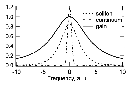
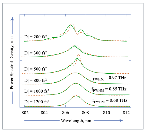
The continuum can be viewed as a long pulse competing with the soliton for the available gain. In the frequency domain, see Figure 6.9, the soliton has a broad spectrum compared to the continuum. Therefore, the continuum experiences the peak of the gain, whereas the soliton spectrum on average experiences less gain. This advantage in gain of the continuum has to be compensated for in the time domain by the saturable absorber response, see Figure 6.8. Whereas for the soliton, there is a balance of the nonlinearity and the dispersion, this is not so for the continuum. Therefore, the continuum is spread by the dispersion into the regions of high absorption. This mechanism has to clean up the gain window following the soliton and caused by the slow recovery of the absorber. As in the case of active modelocking, once the soliton is too short, i.e. a too long net-gain window arises, the loss of the continuum may be lower than the loss of the soliton, see Figure 6.7 and the continuum may break through and destroy the single pulse soliton solution. As a rule of thumb the absorber recovery time can be about 10 times longer than the soliton width. This modelocking principle is especially important for modelocking of lasers with semiconductor saturable absorbers, which show typical absorber recovery times that may range from 100fs-100 ps. Pulses as short as 13fs have been generated with semiconductor saturable absorbers [11]. Figure 6.10 shows the measured spectra from a Ti:sapphire laser modelocked with a saturable absorber for different values for the intra- cavity dispersion. Lowering the dispersion, increases the bandwidth of the soliton and therefore its loss, while lowering at the same time the loss for the continuum. At some value of the dispersion the laser has to become unstabile by break through of the continuum. In the example shown, this occurs at a dispersion value of about \(D = -500fs^2\). The continuum break-through is clearly visible by the additional spectral components showing up at the center of the spectrum. Reducing the dispersion even further might lead again to more stable but complicated spectra related to the formation of higher order solitons. Note the spectra shown are time averaged spectra.

Figure 6.10: Measured (–) and simulated (- - -) spectra from a semiconductor saturable absorber modelocked Ti:sapphire laser for various values of the net intracavity dispersion. Figure by MIT OCW.

Figure 6.11: Measured (–-) and simulated (- - -) autocorrelations corresponding to the spectra shown in Figure 6.10. Figure by MIT OCW.

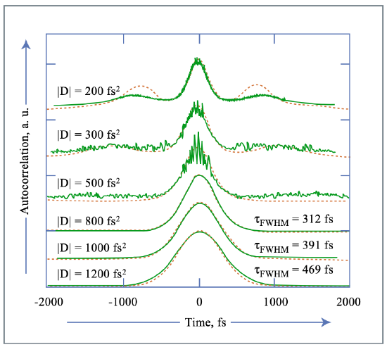
The continuum leads to a background pedestal in the intensity autocorrelation of the emitted pulse, see Figure 6.11. The details of the spectra and autocorrelation may strongly depend on the detailed absorber response.