
10.4: Spectral Interferometry and SPIDER
- Page ID
- 55227
\( \newcommand{\vecs}[1]{\overset { \scriptstyle \rightharpoonup} {\mathbf{#1}} } \)
\( \newcommand{\vecd}[1]{\overset{-\!-\!\rightharpoonup}{\vphantom{a}\smash {#1}}} \)
\( \newcommand{\dsum}{\displaystyle\sum\limits} \)
\( \newcommand{\dint}{\displaystyle\int\limits} \)
\( \newcommand{\dlim}{\displaystyle\lim\limits} \)
\( \newcommand{\id}{\mathrm{id}}\) \( \newcommand{\Span}{\mathrm{span}}\)
( \newcommand{\kernel}{\mathrm{null}\,}\) \( \newcommand{\range}{\mathrm{range}\,}\)
\( \newcommand{\RealPart}{\mathrm{Re}}\) \( \newcommand{\ImaginaryPart}{\mathrm{Im}}\)
\( \newcommand{\Argument}{\mathrm{Arg}}\) \( \newcommand{\norm}[1]{\| #1 \|}\)
\( \newcommand{\inner}[2]{\langle #1, #2 \rangle}\)
\( \newcommand{\Span}{\mathrm{span}}\)
\( \newcommand{\id}{\mathrm{id}}\)
\( \newcommand{\Span}{\mathrm{span}}\)
\( \newcommand{\kernel}{\mathrm{null}\,}\)
\( \newcommand{\range}{\mathrm{range}\,}\)
\( \newcommand{\RealPart}{\mathrm{Re}}\)
\( \newcommand{\ImaginaryPart}{\mathrm{Im}}\)
\( \newcommand{\Argument}{\mathrm{Arg}}\)
\( \newcommand{\norm}[1]{\| #1 \|}\)
\( \newcommand{\inner}[2]{\langle #1, #2 \rangle}\)
\( \newcommand{\Span}{\mathrm{span}}\) \( \newcommand{\AA}{\unicode[.8,0]{x212B}}\)
\( \newcommand{\vectorA}[1]{\vec{#1}} % arrow\)
\( \newcommand{\vectorAt}[1]{\vec{\text{#1}}} % arrow\)
\( \newcommand{\vectorB}[1]{\overset { \scriptstyle \rightharpoonup} {\mathbf{#1}} } \)
\( \newcommand{\vectorC}[1]{\textbf{#1}} \)
\( \newcommand{\vectorD}[1]{\overrightarrow{#1}} \)
\( \newcommand{\vectorDt}[1]{\overrightarrow{\text{#1}}} \)
\( \newcommand{\vectE}[1]{\overset{-\!-\!\rightharpoonup}{\vphantom{a}\smash{\mathbf {#1}}}} \)
\( \newcommand{\vecs}[1]{\overset { \scriptstyle \rightharpoonup} {\mathbf{#1}} } \)
\(\newcommand{\longvect}{\overrightarrow}\)
\( \newcommand{\vecd}[1]{\overset{-\!-\!\rightharpoonup}{\vphantom{a}\smash {#1}}} \)
\(\newcommand{\avec}{\mathbf a}\) \(\newcommand{\bvec}{\mathbf b}\) \(\newcommand{\cvec}{\mathbf c}\) \(\newcommand{\dvec}{\mathbf d}\) \(\newcommand{\dtil}{\widetilde{\mathbf d}}\) \(\newcommand{\evec}{\mathbf e}\) \(\newcommand{\fvec}{\mathbf f}\) \(\newcommand{\nvec}{\mathbf n}\) \(\newcommand{\pvec}{\mathbf p}\) \(\newcommand{\qvec}{\mathbf q}\) \(\newcommand{\svec}{\mathbf s}\) \(\newcommand{\tvec}{\mathbf t}\) \(\newcommand{\uvec}{\mathbf u}\) \(\newcommand{\vvec}{\mathbf v}\) \(\newcommand{\wvec}{\mathbf w}\) \(\newcommand{\xvec}{\mathbf x}\) \(\newcommand{\yvec}{\mathbf y}\) \(\newcommand{\zvec}{\mathbf z}\) \(\newcommand{\rvec}{\mathbf r}\) \(\newcommand{\mvec}{\mathbf m}\) \(\newcommand{\zerovec}{\mathbf 0}\) \(\newcommand{\onevec}{\mathbf 1}\) \(\newcommand{\real}{\mathbb R}\) \(\newcommand{\twovec}[2]{\left[\begin{array}{r}#1 \\ #2 \end{array}\right]}\) \(\newcommand{\ctwovec}[2]{\left[\begin{array}{c}#1 \\ #2 \end{array}\right]}\) \(\newcommand{\threevec}[3]{\left[\begin{array}{r}#1 \\ #2 \\ #3 \end{array}\right]}\) \(\newcommand{\cthreevec}[3]{\left[\begin{array}{c}#1 \\ #2 \\ #3 \end{array}\right]}\) \(\newcommand{\fourvec}[4]{\left[\begin{array}{r}#1 \\ #2 \\ #3 \\ #4 \end{array}\right]}\) \(\newcommand{\cfourvec}[4]{\left[\begin{array}{c}#1 \\ #2 \\ #3 \\ #4 \end{array}\right]}\) \(\newcommand{\fivevec}[5]{\left[\begin{array}{r}#1 \\ #2 \\ #3 \\ #4 \\ #5 \\ \end{array}\right]}\) \(\newcommand{\cfivevec}[5]{\left[\begin{array}{c}#1 \\ #2 \\ #3 \\ #4 \\ #5 \\ \end{array}\right]}\) \(\newcommand{\mattwo}[4]{\left[\begin{array}{rr}#1 \amp #2 \\ #3 \amp #4 \\ \end{array}\right]}\) \(\newcommand{\laspan}[1]{\text{Span}\{#1\}}\) \(\newcommand{\bcal}{\cal B}\) \(\newcommand{\ccal}{\cal C}\) \(\newcommand{\scal}{\cal S}\) \(\newcommand{\wcal}{\cal W}\) \(\newcommand{\ecal}{\cal E}\) \(\newcommand{\coords}[2]{\left\{#1\right\}_{#2}}\) \(\newcommand{\gray}[1]{\color{gray}{#1}}\) \(\newcommand{\lgray}[1]{\color{lightgray}{#1}}\) \(\newcommand{\rank}{\operatorname{rank}}\) \(\newcommand{\row}{\text{Row}}\) \(\newcommand{\col}{\text{Col}}\) \(\renewcommand{\row}{\text{Row}}\) \(\newcommand{\nul}{\text{Nul}}\) \(\newcommand{\var}{\text{Var}}\) \(\newcommand{\corr}{\text{corr}}\) \(\newcommand{\len}[1]{\left|#1\right|}\) \(\newcommand{\bbar}{\overline{\bvec}}\) \(\newcommand{\bhat}{\widehat{\bvec}}\) \(\newcommand{\bperp}{\bvec^\perp}\) \(\newcommand{\xhat}{\widehat{\xvec}}\) \(\newcommand{\vhat}{\widehat{\vvec}}\) \(\newcommand{\uhat}{\widehat{\uvec}}\) \(\newcommand{\what}{\widehat{\wvec}}\) \(\newcommand{\Sighat}{\widehat{\Sigma}}\) \(\newcommand{\lt}{<}\) \(\newcommand{\gt}{>}\) \(\newcommand{\amp}{&}\) \(\definecolor{fillinmathshade}{gray}{0.9}\)Spectral Phase Interferometry for Direct Electric-Field Reconstruction (SPI-DER) avoids iterative reconstruction of the phase profile. Iterative Fourier transform algorithms do have the disadvantage of sometimes being rather time consuming, preventing real-time pulse characterization. In addition, for “pathological" pulse forms, reconstruction is difficult or even impossible. It is mathematically not proven that the retrieval algorithms are unambigu- ous especially in the presence of noise.
Spectral shearing interferometry provides an elegant method to overcome these disadvantages. This technique has been first introduced by C. Iaconis and I.A. Walmsley in 1999 [11] and called spectral phase interferometry for direct electric-field reconstruction - SPIDER. Before we discuss SPIDER lets look at spectral interferometry in general
Spectral Interferometry
The spectrum of a pulse can easily be measured with a spectrometer. The pulse would be completely know, if we could determine the phase across the spectrum. To determine this unknown phase spectral interferometry for pulse measurement has been proposed early on by Froehly and others [12]. If we would have a well referenced pulse with field \(E_R(t)\), superimpose the unknown electric field \(E_S(t)\) delayed with the reference pulse and interfere them in a spectrometer, see Figure 10.21, we obtain for the spectrometer output
\[E_I (t) = E_R (t) + E_s (t - \tau) \nonumber \]
\[\hat{S} (\omega) = \left | \int_{-\infty}^{+\infty} E_I (t) e^{-j \omega t} dt \right |^2 = \left | \hat{E}_R (\omega) + \hat{E}_S (\omega)^{-j \omega \tau} \right |^2 \nonumber \]
\[= \hat{S}_{DC} (\omega) + \hat{S}^{(-)} (\omega) e^{j \omega \tau} + \hat{S}^{(+)} (\omega) e^{-j \omega \tau} \nonumber \]
with
\[\hat{S}^{(+)} (\omega) = \hat{E}_R^* (\omega) \hat{E}_S (\omega) \nonumber \]
\[\hat{S}^{(-)} (\omega) = \hat{S}^{(+)*} (\omega) \nonumber \]
Where (+) and (-) indicate as before, well separted positive and negative "frequency" signals, where "frequency" is now related to \(\tau\) rather than \(\omega\).
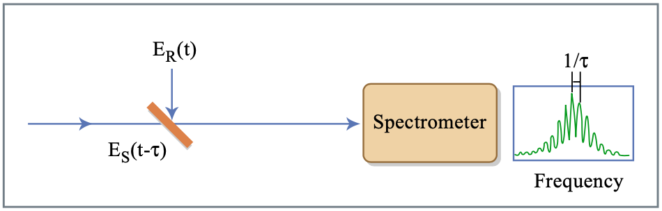
Figure by MIT OCW.
If \(\tau\) is chosen large enough, the inverse Fourier transformed spectrum \(S(t) = F^{-1} \{ \hat{S} (\omega) \}\) results in well separated signals, see Figure 10.22.
\[S(t) = S_{DC} (t) + S^{(-)} (t + \tau) + \hat{S}^{(+)} (t - \tau) \nonumber \]
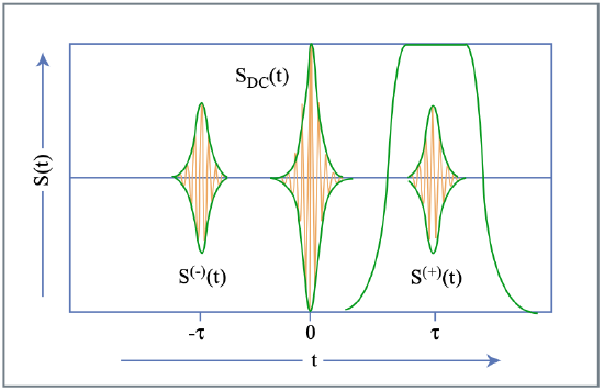
Figure by MIT OCW.
We can isolate either the positive or negative frequency term with a filter in the time domain. Back transformation of the corresponding term to the frequency domain and computation of the spectral phase of one of the terms results in the spectral phase of the signal up to the known phase of the reference pulse and a linear phase contribution from the delay.
\[\Phi^{(+)} (\omega) = \text{arg} \{ \hat{S}^{(+)} (\omega) e^{j \omega \tau} \} = \varphi_S (\omega) -\varphi_R (\omega) + \omega \tau \nonumber \]
SPIDER
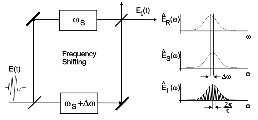
What can we do if we don’t have a well characterized reference pulse? C. Iaconis and I.A. Walmsley [?] came up with the idea of generating two up- converted spectra slightly shifted in frequency and to investigate the spectral interference of these two copies, see Figure 10.23. We use
\[E_R (t) = E(t) e^{j \omega_S t} \nonumber \]
\[E_S (t) = E(t - \tau) e^{j(\omega_S + \Omega) t} \nonumber \]
\[E_I (t) = E_R (t) + E_S (t) \nonumber \]
where \(\omega_s\) and \(\omega_s + \Omega\) are the two frequencies used for upconversion and \(\Omega\) is called the spectral shear between the two pulses. \(E(t)\) is the unknown electric field with spectrum
\[\hat{E} (\omega) = \left |\hat{E} (\omega) \right | e^{j \varphi (\omega)} \nonumber \]
Spectral interferometry using these specially constructed signal and reference pulses results in
\[\hat{S} (\omega) = \left | \int_{-\infty}^{+\infty} E_I (t) e^{-j \omega t} dt \right |^2 = \hat{S}_{DC} (\omega) + \hat{S}^{(-)} (\omega) e^{j \omega \tau} + \hat{S}^{(+)} e^{-j \omega \tau} \nonumber \]
\[\hat{S}^{(+)} (\omega) = \hat{E}_R^* (\omega) \hat{E}_S (\omega) = \hat{E}^* (\omega - \omega_s) \hat{E} (\omega - \omega_s - \Omega) \nonumber \]
\[\hat{S}^{(-)} (\omega) = \hat{S}^{(+)*} (\omega)\label{eq10.4.14} \]
The phase \(\psi (\omega) = \text{arg} [\hat{S}^{(+)} e^{-j \omega \tau}]\) derived from the isolated positive spectral component is
\[\psi (\omega) = \varphi (\omega - \omega_s - \Omega) - \varphi (\omega - \omega_s) - \omega \tau.\label{eq10.4.15} \]
The linear phase \(\omega \tau\) can be substracted off after independent determination of the time delay \(\tau\). It is obvious that the spectral shear \(\Omega\) has to be small compared to the spectral bandwdith \(\Delta \omega\) of the pulse, see Figure 10.23. Then the phase difference in Eq.(\(\ref{eq10.4.13}\)) is proportional to the group delay in the pulse, i.e.
\[-\Omega \dfrac{d\varphi}{d \omega} = \psi (\omega), \nonumber \]
or
\[\varphi (\omega) = -\dfrac{1}{\Omega} \int_{0}^{\omega} \psi (\omega') d\omega'. \nonumber \]
Note, an error \(\Delta \tau\) in the calibration of the time delay \(\tau\) results in an error in the chirp of the pulse
\[\Delta \varphi (\omega) = -\dfrac{\omega^2}{2 \Omega} \Delta \tau.\label{eq10.4.18} \]
Thus it is important to chose a spectral shear \(\Omega\) that is not too small. How small does it need to be? We essentially sample the phase with a sample spacing \(\Omega\). The Nyquist theorem states that we can uniquely resolve a pulse in the time domain if it is only nonzero over a length \([-T, T]\), where \(T = \tau /\Omega\). On the other side the shear \(\Omega\) has to be large enough so that the fringes in the spectrum can be resolved with the available spectrometer.
SPIDER Setup
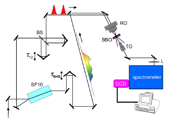
We follow the work of Gallmann et al. [?] that can be used for characteri- zation of pulses only a few optical cycles in duration. The setup is shown in Figure 10.24.
Courtesy of Richard Ell. Used with permission.
Generation of two replica without additional chirp:
A Michelson—type interferometer generates two unchirped replicas. The beam—splitters BS have to be broadband, not to distort the pulses. The delay \(\tau\) between the two replica has to be properly chosen, i.e. in the setup shown it was about 400-500 fs corresponding to 120-150 \(\mu\)m distance in space.
Spectral shearing:
The spectrally sheared copies of the pulse are generated by sum-frequency generation (SFG) with quasi-monochromatic beams at frequencies \(\omega_s\) and \(\omega_s + \Omega\). These quasi monochromatic signals are generated by strong chirp- ing of a third replica (cf. Figure 10.24) of the signal pulse that propagates through a strongly dispersive glass slab. For the current setup we estimate for the broadening of a Gaussian pulse due to the glass dispersion from 5 fs to approximately 6ps. Such a stretching of more than a factor of thousand assures that SFG occurs within an optical bandwidth less than 1 nm, a quasi-monochromatic signal. Adjustment of the temporal overlap \(\tau_{SHG}\) with the two unchirped replica is possible by a second delay line. The streched pulse can be computed by propagation of the signal pulse \(E(t)\) through the strongly dispersive medium with transfer characteristic
\[H_{glass} (omega) = e^{-j D_{glass} (\omega -\omega_c)^2/2} \nonumber \]
neglecting linear group delay and higher order dispersion terms. We otain for the analytic part of the electric field of the streched pulse leaving the glass block by convolution with the transfer characteristic
\[E_{stretch} (t) = \int_{-\infty}^{+\infty} \hat{E} (\omega) e^{-j D_{glass} (\omega - \omega_c)^2/2} e^{j \omega t} d\omega = \nonumber \]
\[= e^{jt^2/(2 D_{glass}) e^{j \omega_c t} \int_{-\infty}^{+\infty} \hat{E} (\omega) e^{-jD_{glass} ((\omega - \omega_c) - t/D_{glass}^2)/2} d \omega \nonumber \]
If the spectrum of the pulse is smooth enough, the stationary phase method can be applied for evaluation of the integral and we obtain
\[E_{stretch} (t) \propto e^{j \omega_c (t + t^2/(2D_{glass})} \hat{E} (\omega = \omega_c + t/D_{glass}) \nonumber \]
Thus the field strength at the position where the instantaneous frequency is
\[\omega_{inst} = \dfrac{d}{dt} \omega_c (t + t^2/(2D_{glass})) = \omega_c + t/D_{glass}\label{eq10.4.23} \]
is given by the spectral amplitude at that frequency, \(\hat{E} (\omega = \omega_c + t/D_{glass})\). For large stretching, i.e.
\[|\tau_p/D_{glass}| \ll |\Omega|\label{eq10.4.24} \]
the up-conversion can be assumed to be quasi monochromatic.
SFG:
A BBO crystal (wedged 10-50\(\mu\)m) is used for type I phase-matched SFG. Type II phase-matching would allow for higher acceptance bandwidths. The pulses are focused into the BBO-crystal by a reflective objective composed of curved mirrors. The signal is collimated by another objective. Due to SFG with the chirped pulse the spectral shear is related to the delay between both pulses, \(\tau\), determined by Eq.(\(\ref{eq10.4.23}\)) to be
\[\Omega = -\tau/ D_{glass}.\label{eq10.4.25} \]
Note, that conditions (\(\ref{eq10.4.24}\)) and (\(\ref{eq10.4.25}\)) are consistent with the fact that the delay between the two pulses should be much larger than the pulse width \(\tau_p\) which also enables the separation of the spectra in Fig.10.22 to determine the spectral phase using the Fourier transform method. For characterization of sub-10fs pulses a crystal thickness around 30μm is a good compromise. Efficiency is still high enough for common cooled CCD-cameras, dispersion is already sufficiently low and the phase matching bandwidth large enough.
Signal detection and phase reconstruction:
An additional lens focuses the SPIDER signal into a spectrometer with a CCD camera at the exit plane. Data registration and analysis is performed with a computer. The initial search for a SPIDER signal is performed by chopping and Lock-In detection.The chopper wheel is placed in a way that the unchirped pulses are modulated by the external part of the wheel and the chirped pulse by the inner part of the wheel. Outer and inner part have dif- ferent slit frequencies. A SPIDER signal is then modulated by the difference (and sum) frequency which is discriminated by the Lock-In amplifier. Once a signal is measured, further optimization can be obtained by improving the spatial and temporal overlap of the beams in the BBO-crystal.
One of the advantages of SPIDER is that only the missing phase informa- tion is extracted from the measured data. Due to the limited phase-matching bandwidth of the nonlinear crystal and the spectral response of grating and CCD, the fundamental spectrum is not imaged in its original form but rather with reduced intensity in the spectral wings. But as long as the interference fringes are visible any damping in the spectral wings and deformation of the spectrum does not impact the phase reconstruction process the SPIDER technique delivers the correct information. The SPIDER trace is then generated by detecting the spectral interference of the pulses
\[E_R (t) = E(t) \hat{E} (\omega_s) e^{j \omega_S t} \nonumber \]
\[E_S (t) = E(t - \tau) \hat{E} (\omega_s + \Omega) e^{j (\omega_S + \Omega) t \nonumber \]
\[E_I (t) = E_R (t) + E_S (t) \nonumber \]
The positive and negative frequency components of the SIDER trace are then according to Eqs.(\(\ref{eq10.4.14}\))
\[\hat{S}^{(+)} (\omega) = \hat{E}_R^* (\omega) \hat{E}_S (\omega) = \hat{E}^* (\omega - \omega_s - \Omega) \hat{E}^* (\omega_s) \hat{E} (\omega_s - \Omega) \nonumber \]
\[\hat{S}^{(-)} (\omega) = \hat{S}^{(+)*} (\omega) \nonumber \]
and the phase \(\psi (\omega) = \text{arg} [\hat{S}^{(+)} (\omega) e^{-j \omega \tau}]\) derived from the isolated positive spectral component substraction already the linear phase off is
\[\psi (\omega) = \varphi (\omega - \omega_s - \Omega) - \varphi (\omega - \oemga_s) - \varphi (\omega - \omega_s - \Omega) + \varphi (\omega_s - \Omega) - \varphi (\omega_s). \nonumber \]
Thus up to an additional constant it delivers the group delay within the pulse to be characterized. A constant group delay is of no physical significance.
SPIDER-Calibration
This is the most critical part of the SPIDER measurement. There are three quantities to be determined with high accuracy and reproducibility:
- delay \(\tau\)
- shift \(\omega_s\)
- shear \(\Omega\)
Delay \(\tau\):
The delay \(\tau\) is the temporal shift between the unchirped pulses. It appears as a frequency dependent phase term in the SPIDER phase, Eqs. (\(\ref{eq10.4.15}\)) and leads to an error in the pulse chirp if not properly substracted out, see Eq.(\(\ref{eq10.4.18}\)).
A determination of \(\tau\) should preferentially be done with the pulses detected by the spectrometer but without the spectral shear so that the observed fringes are all exactly spaced by \(1/\tau\). Such an interferogram may be obtained by blocking the chirped pulse and overlapping of the individual SHG signals from the two unchirped pulses. A Fourier transform of the interferogram delivers the desired delay \(\tau\). In practice, this technique might be difficult to use. Experiment and simulation show that already minor changes of \(\tau\) (\(\pm 1\) fs) significantly alter the reconstructed pulse duration (\(\approx \pm\) 1 - 10%).
Another way for determination of \(\tau\) is the following. As already mentioned, \(\tau\) is accessible by a differentiation of the SPIDER phase with respect to \(\omega\). The delay \(\tau\) therefore represents a constant GDD. An improper determination of \(\tau\) is thus equivalent to a false GDD measurement. The real physical GDD of the pulse can be minimized by a simultaneous IAC measurement. Maximum signal level, respectively shortest IAC trace means an average GDD of zero. The pulse duration is then only limited by higher order dispersion not depending on \(\tau\). After the IAC measurement, the delay \(\tau\) is chosen such that the SPIDER measurement provides the shortest pulse duration. This is justified because through the IAC we know that the pulse duration is only limited by higher order dispersion and not by the GDD \(\propto \tau\). The disadvantage of this method is that an additional IAC setup is needed.
Shift \(\omega_s\):
The SFG process shifts the original spectrum by a frequency \(\omega_s \approx 300\) THz towards higher frequencies equivalent to about 450nm when Ti:sapphire pulses are characterized. If the SPIDER setup is well adjusted, the square of the SPIDER interferogram measured by the CCD is similar to the fundamental spectrum. A determination of the shift can be done by correlating both spectra with each other. Determination of \(\omega_s\) only influences the frequency too which we assign a give phase value, which is not as critical.
Shear \(\Omega\):
The spectral shear is uncritical and can be estimated by the glass dispersion and the delay \(\tau\).
Characterization of Sub-Two-Cycle Ti:sapphire Laser Pulses
The setup and the data registration and processing can be optimized such that the SPIDER interferogram and the reconstructed phase, GDD and intensity envelope are displayed on a screen with update rates in the range of 0.5-1s.
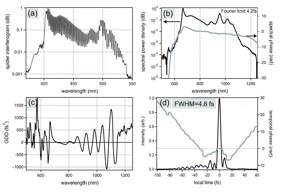
Real-time SPIDER measurements enabled the optimization of external dispersion compensation leading to 4.8 fs pulses directly from a laser [13], see Figure 10.25.
Courtesy of Richard Ell. Used with permission.
Figure 10.25(a) shows the SPIDER interferogram as detected by the CCD camera. The interferogram is modulated up to 90%, the resolutions limit in the displayed graphic can not resolve this. The large number of interference fringes assures reliable phase calculation. Figure (b) displays the laser spectrum registered by the optical spectrum analyzer on a logarithmic scale. The calculated spectral phase curve is added in this plot. The small slope of the phase curve corresponds to a constant GD which is an unimportant time shift. Figure 10.25 (c) depicts the GDD obtained from the phase by two derivatives with respect to the angular frequency \(\omega\). The last Figure (d) shows the intensity envelope with a FWHM pulse duration of 4.8 fs together with the temporal phase curve.
Pros and Cons of SPIDER
| Advantages | Disadvantages |
| direct analytical phase extraction | complex experimental setup |
| no moving mirrors or other components | precise delay calibration necessary |
| possible real-time characterization | "compact" spectrum necessary (no zero-intensity intervals) |
| simple 1-D data acquisition | need for expensibve CCD-camera |
| minor dependence on spectral response of nonlinear crystal and spectrometer |
Bibliography
[1] K. Naganuma, K. Mogi, H. Yamada, "General method for ultrashort light pulse chirp measurement," IEEE J. of Quant. Elec. 25, 1225 - 1233 (1989).
[2] J. C. Diels, J. J. Fontaine, and F. Simoni, "Phase Sensitive Measurement of Femtosecond Laser Pulses From a Ring Cavity," in Proceedings of the International Conf. on Lasers. 1983, STS Press: McLean, VA, p. 348-355. J. C. Diels et al.,"Control and measurement of Ultrashort Pulse Shapes (in Amplitude and Phase) with Femtosecond Accuracy," Applied Optics 24, 1270-82 (1985).
[3] J.W. Nicholson, J.Jasapara, W. Rudolph, F.G. Ometto and A.J. Taylor, "Full-field characterization of femtosecond pulses by spectrum and cross- correlation measurements, "Opt. Lett. 24, 1774 (1999).
[4] D. T. Reid, et al., Opt. Lett. 22, 233-235 (1997).
[5] R. Trebino, "Frequency-Resolved Optical Gating: the Measurement of
Ultrashort Laser Pulses,"Kluwer Academic Press, Boston, (2000).
[6] Trebino, et al., Rev. Sci. Instr., 68, 3277 (1997).
[7] Kane and Trebino, Opt. Lett., 18, 823 (1993).
[8] Stark, Image Recovery, Academic Press, 1987.
[9] L. Cohen, "Time-frequency distributions-a review, " Proceedings of the IEEE, 77, 941 - 981 (1989).
[10] L. Gallmann, D. H. Sutter, N. Matuschek, G. Steinmeyer and U. Keller, "Characterization of sub-6fs optical pulses with spectral phase inter- ferometry for direct electric-field reconstruction," Opt. Lett. 24, 1314 (1999).
[11] C. Iaconis and I. A. Walmsley, Self-Referencing Spectral Interferometry for Measuring Ultrashort Optical Pulses, IEEE J. of Quant. Elec. 35, 501 (1999).
[12] C. Froehly, A. Lacourt, J. C. Vienot, "Notions de reponse impulsionelle et de fonction de tranfert temporelles des pupilles opticques, justifica- tions experimentales et applications," Nouv. Rev. Optique 4, 18 (1973).
[13] Richard Ell, "Sub-Two Cycle Ti:sapphire Laser and Phase Sensitive Nonlinear Optics," PhD-Thesis, University of Karlsruhe (TH), (2003).