
10.3: Frequency Resolved Optical Gating (FROG)
- Page ID
- 44681

We follow closely the bock of the FROG inventor Rich Trebino. In frequency resolved optical gating, the pulse to be characterized is gated by another ultrashort pulse [5]. The gating is no simple linear sampling technique, but the pulses are crossed in a medium with an instantaneous nonlinearity (\(\chi (2)\) or \(\chi (3)\)) in the same way as in an autocorrelation measurement (Figures 10.1 and 10.10). The FROG—signal is a convolution of the unknown electric-field \(E(t)\) with the gating-field \(g(t)\) (often a copy of the unknown pulse itself). However, after the interaction of the pulse to be measured and the gate pulse, the emitted nonlinear optical radiation is not put into a simple photo detector, but is instead spectrally resolved detected. The general form of the frequency-resolved intensity, or Spectrogram \(S_F (\tau, \omega)\) is given by
\[S_F (\tau, \omega) \propto \left|\int_{-\infty}^{\infty} E(t) \cdot g(t - \tau) e^{-j \omega t} dt \right|^2\label{eq10.3.1} \]
Image removed due to copyright considerations.
Figure 10.10: The spectrogram of a waveform E(t) tells the intensity and frequency in a given time interval [5].
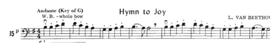
Representations of signals, or waveforms in general, by time-frequency distributions has a long history. Most notably musical scores are a temporal sequence of tones giving its frequency and volume, see Figure 10.11.
Time-frequency representations are well known in the radar community, signal processing and quantum mechanics [9] (Spectrogram, Wigner-Distribution, Husimi-Distribution, ...), Figure 10.12 shows the spectrogram of differently chirped pulses. Like a musical score, the spectrogram visually displays the frequency vs. time.
Image removed due to copyright considerations.
Figure 10.12: Like a musical score, the spectrogram visually displays the frequency vs. time [5].
Note, that the gate pulse in the FROG measurement technique does not to be very short. In fact if we have
\[g(t) \equiv \delta (t) \nonumber \]
then
\[S_F (\tau, \omega) = |E(\tau)|^2 \nonumber \]
and the phase information is completely lost. There is no need for short gate pulses. A gate length of the order of the pulse length is sufficient. It temporally resolves the slow components and spectrally the fast components.
Polarization Gate FROG
Figure 10.13 shows the setup [6][7]. FROG is based on the generation of a well defined gate pulse, eventually not yet known. This can be achieved by using the pulse to be measured and an ultrafast nonlinear interaction. For example the electronic Kerr effect can be used to induce an ultrafast polarization modulation, that can gate the pulse with a copy of the same pulse.
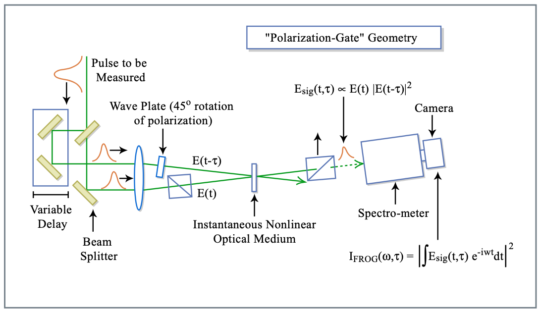
The signal analyzed in the FROG trace is, see Figure 10.14,
\[E_{sig} (t, \tau) = E(t) |E(t - \tau)|^2\label{eq10.3.4} \]
Image removed due to copyright considerations.
Figure 10.14: The signal pulse reflects the color of the gated pulse at the time \(2\tau/3\) [5]
The FROG traces generated from a PG-FROG for chirped pulses is identical to Figure 10.12. Figure 10.15 shows FROG traces of more complicated pulses
Image removed due to copyright considerations.
Figure 10.15: FROG traces of more complicated pulses.
FROG Inversion Algorithm
Spectrogram inversion algorithms need to know the gate function \(g(t - \tau)\), which in the given case is related to the yet unknown pulse. So how do we get from the FROG trace to the pulse shape with respect to amplitude and phase? If there is such an algorithm, which produces solutions, the question of uniqueness of this solution arises. To get insight into these issues, we realize, that the FROG trace can be written as
\[I_{FROG} (\tau, \omega) \propto \left|\int_{-\infty}^{\infty} E_{sig} (t, \tau) e^{-j \omega t} dt \right|^2 \nonumber \]
Writing the signal field as a Fourier transform in the time variable, i.e.
\[E_{sig} (t, \tau) = \int_{-\infty}^{\infty} \hat{E}_{sig} (t, \Omega) e^{-j \Omega \tau} d \Omega \nonumber \]
yields
\[I_{FROG} (\tau, \omega) \propto \left|\int_{-\infty}^{\infty} \hat{E}_{sig} (t, \Omega) e^{-j \omega t - j \Omega \tau} dt d\Omega \right|^2.\label{eq10.3.7} \]
This equation shows that the FROG-trace is the magnitude square of a two-dimensional Fourier transform related to the signal field \(E_{sig}(t,\tau)\). The inversion of Eq.(\(\ref{eq10.3.7}\)) is known as the 2D-phase retrival problem. Fortunately algorithms for this inversion exist [8] and it is known that the magnitude (or magnitude square) of a 2D-Fourier transform (FT) essentially uniquely determines also its phase, if additional conditions, such as finite support or the relationship (\(\ref{eq10.3.4}\)) is given. Essentially unique means, that there are ambiguities but they are not dense in the function space of possible 2D-transforms, i.e. they have probability zero to occur.
Furthermore, the unknown pulse \(E(t)\) can be easily obtained from the modified signal field \(\hat{E}_{sig} (t,\Omega)\) because
\[\begin{align*} \hat{E}_{sig} (t, \Omega) &= \int_{-\infty}^{\infty} E_{sig} (t, \tau) e^{j \Omega \tau} d \tau
\\[4pt] &= \int_{-\infty}^{\infty} E(t) g(t - \tau) e^{-j\Omega \tau} d\tau
\\[4pt] &= E(t) G^* (\Omega) e^{-j\Omega t} \end{align*} \nonumber \]
with
\[G(\Omega) = \int_{-\infty}^{\infty} g(\tau) e^{-\Omega \tau} d\tau. \nonumber \]
Thus there is
\[E(t) \propto \hat{E}_{sig} (t, 0). \nonumber \]
The only condition is that the gate function should be chosen such that \(G(\Omega) \ne 0\). This is very powerful.
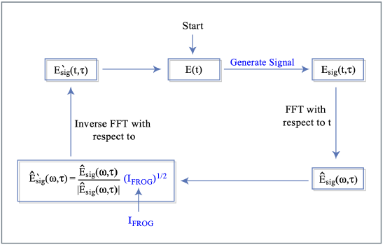
Fourier Transform Algorithm
The Fourier transform algorithm also commonly used in other phase retrieval problems is schematically shown in Figure 10.16
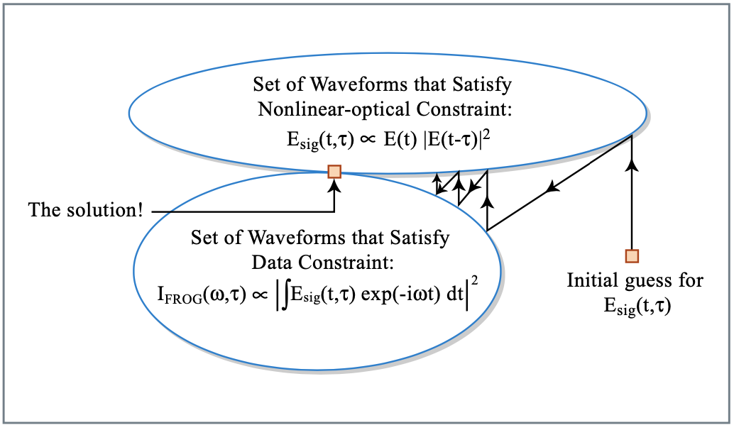
Generalized Projections
The signal field \(E_{sig}(t, \tau)\) has to fulfill two constraints, which define sets see Figure 10.17. The intersection between both sets results in yields \(E(t)\). Moving to the closest point in one constraint set and then the other yields convergence to the solution, if the two sets or convex. Unfortunately, the FROG constraints are not convex. Nevertheless the algorithm works surprisingly well. For more information consult with reference [5].
Second Harmonic FROG
So far we only discussed PG-FROG. However, if we choose a \(\chi^{(2)}\) nonlinearity, e.g. SHG, and set the gating-field equal to a copy of the pulse \(g(t) \equiv E(t)\), we are measuring in eq.(\(\ref{eq10.3.1}\)) the spectrally resolved autocorrelation signal. The marginals of the measured FROG-trace do have the following properties
\[\int_{-\infty}^{\infty} S_F (\tau, \omega) d\omega \propto \int_{-\infty}^{\infty} |E(t)|^2 \cdot |g(t - \tau)|^2 dt = I_{AC} (\tau). \nonumber \]
\[\int_{-\infty}^{\infty} S_F (\tau, \omega) d\tau \propto \left|\int_{-\infty}^{\infty} \hat{E} (\omega) \cdot \hat{G} (\omega - \omega')^2 d\omega' \right| = \left|\hat{E}_{2\omega} (\omega) \right|^2. \nonumber \]
For the case, where \(g(t) \equiv E(t)\), we obtain
\[\int_{-\infty}^{\infty} S_F (\tau, \omega) d\omega \propto I_{AC} (\tau). \nonumber \]
\[\int_{-\infty}^{\infty} S_F (\tau, \omega) d \tau \propto \left | \hat{E}_{2\omega} (\omega)\right |^2. \nonumber \]
The setup to measure the Frog-trace is identical with the setup to measure the intensity autocorrelation function (Figure 10.1) only the photodector for the second harmonic is replaced by a spectrometer (Figure 10.18).
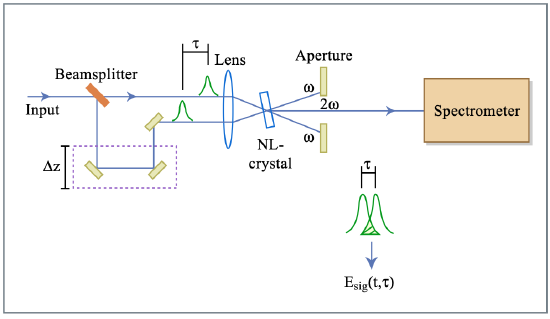
Figure by MIT OCW.
Since the intensity autocorrelation function and the integrated spectrum can be measured simultaneously, this gives redundancy to check the correctness of all measurements via the marginals (10.38, 10.39). Figure 10.19 shows the SHG-FROG trace of the shortest pulses measured sofar with FROG.
Image removed due to copyright restrictions. Please see:
Baltuska, Pshenichnikov, and Wiersma. Journal of Quantum Electronics 35 (1999): 459.
Figure 10.19: FROG measurement of a 4.5 fs laser pulse.
FROG Geometries
The Frog-signal Esig .can also be generated by a nonlinear interaction different from SHG or PG, see table 10.20[5].
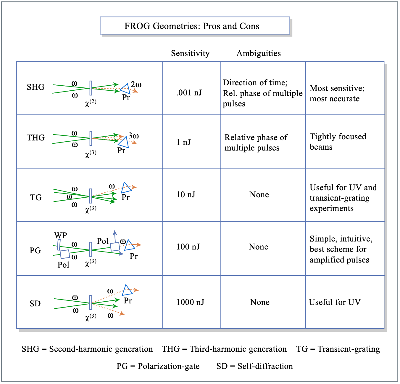
Figure by MIT OCW.