10.2: Interferometric Autocorrelation (IAC)

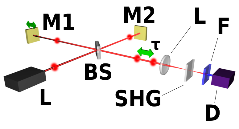
A pulse characterization method, that also reveals the phase of the pulse is the interferometric autocorrelation introduced by J. C. Diels [2], (Figure 10.2 a). The input beam is again split into two and one of them is delayed. However, now the two pulses are sent colinearly into the nonlinear crystal. Only the SHG component is detected after the filter.

Figure 10.2: (a) Setup for an interferometric autocorrelation. Setup for an interferometric autocorrelator, similar to the field autocorrelator above, with the following optics added: L: converging lens, SHG: second-harmonic generation crystal, F: spectral filter to block the fundamental wavelength. (CC BY-SA 3.0; via Wikipedia) (b) Delay stage, so that both beams are reflected from the same air/medium interface imposing the same phase shifts on both pulses.

The total field \(E(t,\tau)\) after the Michelson-Interferometer is given by the two identical pulses delayed by \(\tau\) with respect to each other

\[\begin{align*}E(t, \tau) &= E(t + \tau) + E(t) \\[4pt] &= A(t + \tau) e^{j\omega_c (t + \tau)} e^{j \phi_{CE}} + A(t) e^{j \omega_c t} e^{j \phi_{CE}}. \end{align*} \nonumber \]

A(t) is the complex amplitude, the term \(e^{i\omega_0 t}\) describes the oscillation with the carrier frequency \(\omega_0\) and \(\phi_{CE}\) is the carrier-envelope phase. Equation (10.1.1) writes

\[P^{(2)} (t, \tau) \propto (A(t + \tau) e^{j \omega_c (t + \tau)} e^{j \phi_{CE}} + A(t) e^{j \omega_c t} e^{j\phi_{CE}})^2 \nonumber \]

This is only idealy the case if the paths for both beams are identical. If for example dielectric or metal beamsplitters are used, there are different reflections involved in the Michelson-Interferometer shown in Figure 10.2 (a) leading to a differential phase shift between the two pulses. This can be avoided by an exactly symmetric delay stage as shown in Figure 10.1 (b).

Again, the radiated second harmonic electric field is proportional to the polarization

\[E(t, \tau) \propto (A(t + \tau) e^{j \omega_c (t + \tau)} e^{j \phi_{CE}} + A(t) e^{j \omega_c t} e^{j\phi_{CE}})^2 \nonumber \]

The photo—detector (or photomultiplier) integrates over the envelope of each individual pulse

\[\begin{array} {rcl} {I(\tau)} & \propto & {\int_{-\infty}^{\infty} |(A(t + \tau) e^{j\omega_c (t + \tau)} + A(t) e^{j\omega_c t})^2|^2 dt.} \\ {} & \propto & {\int_{-\infty}^{\infty} |A^2(t + \tau) e^{j 2 \omega_c (t + \tau)} + 2A(t + \tau) A(t) e^{j\omega_c (t + \tau)} e^{j \omega_c t} + A^2 (t) e^{j 2 \omega_c t}|^2.} \end{array} \nonumber \]

Evaluation of the absolute square leads to the following expression

\[\begin{array} {rcl} {I(\tau)} & \propto & {\int_{-\infty}^{\infty} [|A(t + \tau)|^4 + 4|A(t + \tau)|^2 |A(t)|^2 + |A(t)|^4} \\ {} & \ & {+2A(t + \tau) |A(t)|^2 A^* (t) e^{j \omega_c \tau} + c.c.} \\ {} & \ & {+2A(t)|A(t + \tau)|^2 A^* (t + \tau) e^{-j \omega_c \tau} + c.c.} \\ {} & \ & {+A^2 (t + \tau) (A^* (t))^2 e^{j2\omega_c \tau} + c.c.]dt.} \end{array} \nonumber \]

The carrier—envelope phase \(\phi_{CE}\) drops out since it is identical to both pulses. The interferometric autocorrelation function is composed of the following terms

\[I(\tau) = I_{back} + I_{int} (\tau) + I_{\omega} (\tau) + I_{2 \omega} (\tau). \label{eq10.2.7} \]

Background signal \(I_{back}\):

\[I_{back} = \int_{-\infty}^{\infty} (|A(t + \tau)|^4 + |A(t)|^4) dt = 2 \int_{-\infty}^{\infty} I^2 (t) dt \nonumber \]

Intensity autocorrelation \(I_{int} (\tau)\):

\[I_{int} (\tau) = 4\int_{-\infty}^{\infty} |A(t + \tau)|^2 |A(t)|^2 dt = 4 \int_{-\infty}^{\infty} I(t + \tau) \cdot I(t) dt \nonumber \]

Coherence term oscillating with \(\omega_c\): \(I_{\omega} (\tau)\):

\[I_{\omega} (\tau) = 4 \int_{-\infty}^{\infty} \text{Re} [(I(t) + I(t + \tau)) A^* (t) A(t + \tau) e^{j \omega \tau}] dt \nonumber \]

Coherence term oscillating with \(2 \omega_c\): \(I_{2\omega} (\tau)\):

\[I_{\omega} (\tau) = 2 \int_{-\infty}^{\infty} \text{Re} [A^2 (t) (A^* (t + \tau))^2 e^{j2\omega \tau}] dt \nonumber \]

Equation (\(\ref{eq10.2.7}\)) is often normalized relative to the background intensity Iback resulting in the interferometric autocorrelation trace

\[I_{IAC} (\tau) = 1 + \dfrac{I_{int}(\tau)}{I_{back}} + \dfrac{I_{\omega}(\tau)}{I_{back}} + \dfrac{I_{2 \omega}(\tau)}{I_{back}}.\label{eq10.2.12} \]

Equation (\(\ref{eq10.2.12}\)) is the final equation for the normalized interferometric auto- correlation. The term \(I_{int} (\tau)\) is the intensity autocorrelation, measured by non—colinear second harmonic generation as discussed before. Therefore, the averaged interferometric autocorrelation results in the intensity autocorrelation sitting on a background of 1.

Figure 10.3 shows a calculated and measured IAC for a sech-shaped pulse.

Image removed due to copyright restrictions.Please see:Keller, U., Ultrafast Laser Physics, Institute of Quantum Electronics, Swiss Federal Institute of Technology, ETH Hönggerberg—HPT, CH-8093 Zurich, Switzerland.

Figure 10.3: Computed and measured interferometric autocorrelation traces for a 10 fs long sech-shaped pulse.

As with the intensity autorcorrelation, by construction the interferometric autocorrelation has to be also symmetric:

\[I_{IAC} (\tau) = I_{IAC} (-\tau). \nonumber \]

This is only true if the beam path between the two replicas in the setup are completely identical, i.e. there is not even a phase shift between the two pulses. A phase shift would lead to a shift in the fringe pattern, which shows up very strongly in few-cycle long pulses. To avoid such a symmetry breaking, one has to arrange the delay line as shown in Figure 10.2 b so that each pulse travels through the same amount of substrate material and undergoes the same reflections.

At \(\tau = 0\), all integrals are identical

\[\begin{array} {rcl} {I_{back}} & \equiv & {2 \int |A(t)|^4 dt} \\ {I_{int} (\tau = 0)} & \equiv & {2 \int |A^2(t)|^2 dt = 2 \int |A(t)|^4 dt = I_{back}} \\ {I_{\omega} (\tau = 0)} & \equiv & {2 \int |A(t)|^2 A(t) A^* (t) dt = 2 \int |A(t)|^4 dt = I_{back}}\\ {I_{2\omega} (\tau = 0)} & \equiv & {2\int A^2 (t) A^2 (t)^* dt = 2\int |A(t)|^4 dt = I_{back}} \end{array} \nonumber \]

Then, we obtain for the interferometric autocorrelation at zero time delay

\[\begin{array} {l} {I_{IAC} (\tau) |_{\max} = I_{IAC} (0) = 8} \\ {I_{IAC} (\tau \to \pm \infty) = 1} \\ {I_{IAC} (\tau) |_{\min} = 0} \end{array} \nonumber \]

This is the important 1:8 ratio between the wings and the pick of the IAC, which is a good guide for proper alignment of an interferometric autocorrelator. For a chirped pulse the envelope is not any longer real. A chirp in the pulse results in nodes in the IAC. Figure 10.4 shows the IAC of a chirped sech-pulse

\[A(t) = \left ( \text{sech} \left (\dfrac{t}{\tau_p}\right) \right )^{(1 + j\beta)}\nonumber \]

for different chirps.

Image removed due to copyright restrictions.

Please see:
Keller, U., Ultrafast Laser Physics, Institute of Quantum Electronics, Swiss Federal Institute of Technology, ETH Hönggerberg—HPT, CH-8093 Zurich, Switzerland.

Figure 10.4: Influence of increasing chirp on the IAC.

Interferometric Autocorrelation of an Unchirped Sech-Pulse

Envelope of an unchirped sech-pulse

\[A(t) = \text{sech} (t/\tau_p) \nonumber \]

Interferometric autocorrelation of a sech-pulse

\[I_{IAC} (\tau) = 1 + \{2 + \cos (2 \omega_c \tau) \} \dfrac{3((\tfrac{\tau}{\tau_p}) \cosh (\tfrac{\tau}{\tau_p}) - \sinh (\tfrac{\tau}{\tau_p}))}{\sinh^3 (\tfrac{\tau}{\tau_p})} + \dfrac{3(\sinh (\tfrac{2\tau}{\tau_p}) - (\tfrac{2\tau}{\tau_p}))}{\sinh^3 (\tfrac{\tau}{\tau_p})} \cos (\omega_c \tau) \nonumber \]

Interferometric Autocorrelation of a Chirped Gaussian Pulse

Complex envelope of a Gaussian pulse

\[A(t) = \exp \left [-\dfrac{1}{2} \left (\dfrac{t}{t_p} \right ) (1 + j \beta) \right ]. \nonumber \]

Interferometric autocorrelation of a Gaussian pulse

\[I_{IAC} (\tau) = 1 + \{2 + e^{-\tfrac{\beta^2}{2} (\tfrac{\tau}{\tau_p})^2} \cos (2 \omega_c \tau) \} e^{-\tfrac{1}{2} (\tfrac{\tau}{\tau_p})^2} + 4e^{-\tfrac{3+\beta^2}{8} (\tfrac{\tau}{\tau_p})^2} \cos \left (\dfrac{\beta}{4} \left (\dfrac{\tau}{\tau_p} \right )^2 \right ) \cos (\omega_c \tau). \nonumber \]

Second Order Dispersion

It is fairly simple to compute in the Fourier domain what happens in the presence of dispersion.

\[E(t) = A(t) e^{j \omega_c t} \to \tilde{E} (\omega) \nonumber \]

After propagation through a dispersive medium we obtain in the Fourier domain.

\[\tilde{E}' (\omega) = \tilde{E} (\omega) e^{-i\Phi (\omega)}\nonumber \]

and

\[E'(t) = A'9t) e^{j \omega_c t}\nonumber \]

Figure 10.5 shows the pulse amplitude before and after propagation through a medium with second order dispersion. The pulse broadens due to the dispersion. If the dispersion is further increased the broadening increases and the interferometric autocorrelation traces shown in Figure 10.5 develope a characteristic pedestal due to the term \(I_{int}\). The width of the interferomet- rically sensitive part remains the same and is more related to the coherence time in the pulse, that is proportional to the inverse spectral width and does not change.

Image removed due to copyright restrictions.

Please see:
Keller, U., Ultrafast Laser Physics, Institute of Quantum Electronics, Swiss Federal Institute of Technology, ETH Hönggerberg—HPT, CH-8093 Zurich, Switzerland.

Figure 10.5: Effect of various amounts of second order dispersion on a trans- form limited 10 fs Sech-pulse.

Third Order Dispersion

We expect, that third order dispersion affects the pulse significantly for

\[\dfrac{D_3}{\tau^3} > 1\nonumber \]

which is for a 10fs sech-pulse \(D_3 > (\tfrac{10fs}{1.76})^3 183 fs^3\). Figure 10.6 and 10.7 show the impact on pulse shape and interferometric autocorrelation. The odd dispersion term generates asymmetry in the pulse. The interferometric autocorrelation developes characteristic nodes in the wings.

Image removed due to copyright restrictions.

Please see:

Keller, U., Ultrafast Laser Physics, Institute of Quantum Electronics, Swiss Federal Institute of Technology, ETH Hönggerberg—HPT, CH-8093 Zurich, Switzerland.

Figure 10.6: Impact of 200 \(fs^3\) third order dispersion on a 10 fs pulse at a center wavelength of 800 nm.and its interferometric autocorrelation.

Image removed due to copyright restrictions.

Please see:
Keller, U., Ultrafast Laser Physics, Institute of Quantum Electronics, Swiss Federal Institute of Technology, ETH Hönggerberg—HPT, CH-8093 Zurich, Switzerland.

Figure 10.7: Changes due to increasing third order Dispersion from 100-1000 \(fs^3\) on a 10 fs pulse at a center wavelength of 800 nm.

Self-Phase Modulation

Self-phase modulation without compensation by proper negative dispersion generates a phase over the pulse in the time domain. This phase is invisible in the intensity autocorrelation, however it shows up clearly in the IAC, see Figure 10.8 for a Gaussian pulse with a peak nonlinear phase shift \(\phi_0 = \delta A_0^2 = 2\) and Figure 10.8 for a nonlinear phase shift \(\phi_0 = 3\).

Image removed due to copyright restrictions.

Please see:
Keller, U., Ultrafast Laser Physics, Institute of Quantum Electronics, Swiss Federal Institute of Technology, ETH Hönggerberg—HPT, CH-8093 Zurich, Switzerland.

Figure 10.8: Change in pulse shape and interferometric autocorrelation in a 10 fs pulse at 800 nm subject to pure self-phase modulation leading to a nonlinear phase shift of \(\phi_0 = 2\).

Image removed due to copyright restrictions.

Please see:
Keller, U., Ultrafast Laser Physics, Institute of Quantum Electronics, Swiss Federal Institute of Technology, ETH Hönggerberg—HPT, CH-8093 Zurich, Switzerland.

Figure 10.9: Change in pulse shape and interferometric autocorrelation in a 10 fs pulse at 800 nm subject to pure self-phase modulation leading to a nonlinear phase shift of \(\phi_0 = 3\).

From the expierence gained by looking at the above IAC-traces for pulses undergoing second and third order dispersions as well as self-phase modulation we conclude that it is in general impossible to predict purely by looking at the IAC what phase perturbations a pulse might have. Therefore, it was always a wish to reconstruct uniquely the electrical field with respect to amplitude and phase from the measured data. In fact one can show rigorously, that amplitude and phase of a pulse can be derived uniquely from the IAC and the measured spectrum up to a time reversal ambiguityn [1]. Furthermore, it has been shown that a cross-correlation of the pulse with a replica chirped in a known medium and the pulse spectrum is enough to reconstruct the pulse [3]. Since the spectrum of the pulse is already given only the phase has to be determined. If a certain phase is assumed, the electric field and the measured cross-correlation or IAC can be computed. Minimization of the error between the measured cross-correlation or IAC will give the de- sired spectral phase. This procedure has been dubbed PICASO (Phase and Intenisty from Cross Correlation and Spectrum Only).

Note, also instead of measuring the autocorrelation and interferometric autocorrelation with SHG one can also use two-photon absorption or higher order absorption in a semiconductor material (Laser or LED) [4].

However today, the two widely used pulse chracterization techniques are Frequency Resolved Optical Gating (FROG) and Spectral Phase Interferom- etry for Direct Electric Field Reconstruction (SPIDER)