11.4: Four-Wave Mixing

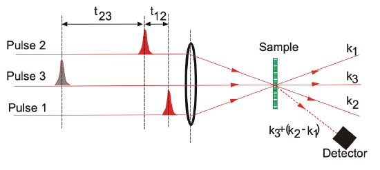
A more advanced ultrafast spectroscopy technique than pump-probe is four- wave mixing (FWM). It enables to investigate not only energy relaxation processes, as is the case in pump-probe measurements, but also dephasing processes in homogenous as well as inhomogenously broadened materials. The typical set-up is shown in Figure 11.12

Figure 11.12: Typical Four-Wave-Mixing (FWM) beam geometry.

Lets assume these pulses interact resonantely with a two-level system modelled by the Bloch Equations derived in chapter 2 (2.1592.162).

\[\left (\Delta - \dfrac{1}{c_0^2} \dfrac{\partial^2}{\partial t^2} \right ) \vec{E}^{(+)} (z, t) = \mu_0 \dfrac{\partial^2}{\partial t^2} \vec{P}^{(+)} (z, t), \nonumber \]

\[\vec{P}^{(+)} (z, t) = -2N \vec{M}^* d(z, t) \nonumber \]

\[\dot{d} (z, t) = -(\dfrac{1}{T_2} - j \omega_{eg})d + \dfrac{1}{2j \hbar} \vec{M} \vec{E}^{(+)} w, \nonumber \]

\[\dot{w} (z, t) = -\dfrac{w - w_0}{T_1} + \dfrac{1}{j \hbar} (\vec{M}^* \vec{E}^{(-)} d - \vec{M} \vec{E}^{(+)} d^*) \nonumber \]

The two-level system, located at \(z = 0\), will be in the ground state, i.e. \(d(t = 0) = 0\) and \(w(t = 0) = -1\), before arrival of the first pulses. That is, no polarization is yet present. Lets assume the pulse interacting with the two-level system are weak and we can apply perturbation theory. Then the arrival of the first pulse with the complex field

\[\vec{E}^{(+)} (\vec{x}, t) = \vec{E}_0^{(+)} \delta (t) e^{j(\omega_{eg} t - j \vec{k}_1 \vec{x})} \nonumber \]

will generate a polarization wave according to the Bloch-equations

\[d(\vec{x}, t) = -\dfrac{\vec{M} \vec{E}_0^{(+)}}{2j \hbar} e^{j(\omega_{eg} - 1/T_2)t} e^{-j \vec{k}_1 \vec{x}} \delta (z), \nonumber \]

which will decay with time. Once a polarization is created the second pulse will change the population and induce a weak population grating

\[\Delta w(\vec{x}, t) = \dfrac{|\vec{M} \vec{E}_0^{(+)}|^2}{\hbar^2} e^{-t_{12}/T_2} e^{-j(\vec{k}_1 - \vec{k}_2)\vec{x}} e^{-(t - t_2)/T_1} \delta (z) + c.c., \nonumber \]

When the third pulse comes, it will scatter of from this population grating, i.e. it will induce a polarization, that radiates a wave into the direction \(\vec{k}_3 + \vec{k}_2 - \vec{k}_1\) according to

\[d (\vec{x}, t) = \dfrac{\vec{M} \vec{E}_0^{(+)}}{2j \hbar} \dfrac{|\vec{M} \vec{E}_0^{(+)}|^2}{\hbar^2} e^{-t_{12}/T_2} e^{-t_{32}/T_1} e^{-j(\vec{k}_3 + \vec{k}_2 - \vec{k}_1)\vec{x}} \delta (z) \nonumber \]

Thus the signal detected in this direction, see Figure 11.12, which is proportional to the square of the radiating dipole layer

\[S(t) \sim |d(\vec{x}, t)|^2 \sim e^{-2t_{12}/T_2} e^{-2t_{32}/T_1} \nonumber \]

will decay on two time scales. If the time delay between pulses 1 and 2, \(t_{12}\), is only varied it will decay with the dephasing time \(T_2/2\). If the time delay between pulses 2 and 3 is varied, \(t_{32}\), the signal strength will decay with the energy relaxation time \(T_1/2\)

Bibliography

[1]  K. L. Hall, G. Lenz, E. P. Ippen, and G. Raybon, "Heterodyne pump- probe technique for time-domain studies of optical nonlinearities in waveguides," Opt. Lett. 17, p.874-876, (1992).

[2]  K. L. Hall, A. M. Darwish, E. P. Ippen, U. Koren and G. Raybon, "Fem- tosecond index nonlinearities in InGaAsP optical amplifiers," App. Phys. Lett. 62, p.1320-1322, (1993).

[3]  K. L. Hall, G. Lenz, A. M. Darwish, E. P. Ippen, "Subpicosecond gain and index nonlinearities in InGaAsP diode lasers," Opt. Comm. 111, p.589-612 (1994).

[4]  J. A. Valdmanis, G. Mourou, and C. W. Gabel, “Picosecond electro-optic sampling system,” Appl. Phys. Lett. 41, p. 211-212 (1982).

[5]  B. H. Kolner and D. M. Bloom, "Electrooptic Sampling in GaAs Inte- grated Circuits," IEEE J. Quantum Elect.22, 79-93 (1986).

[6]  S. Gupta, M. Y. Frankel, J. A. Valdmanis, J. F. Whitaker, G. A. Mourou, F. W. Smith and A. R. Calaw , "Subpicosecond carrier lifetime in GaAs grown by molecular beam epitaxy at low temperatures," App. Phys. Lett. 59, pp. 3276-3278 91991)

[7]  Ch. Fattinger, D. Grischkowsky, "Terahertz beams," Appl. Phys. Lett. 54, pp.490-492 (1989)

[8]  D. M. Mittleman, R. H. Jacobsen, and M. Nuss, "T-Ray Imaging," IEEE JSTQE 2, 679-698 (1996)

[9]  A. Bonvalet, J. Nagle, V. Berger, A. Migus, JL Martin, and M. Joffre, "Ultrafast Dynamic Control of Spin and Charge Density Oscillations in a GaAs Quantum Well," Phys. Rev. Lett. 76, 4392 (1996).