4.4: Antenna Characteristics
- Page ID
- 18960

\( \newcommand{\vecs}[1]{\overset { \scriptstyle \rightharpoonup} {\mathbf{#1}} } \)
\( \newcommand{\vecd}[1]{\overset{-\!-\!\rightharpoonup}{\vphantom{a}\smash {#1}}} \)
\( \newcommand{\dsum}{\displaystyle\sum\limits} \)
\( \newcommand{\dint}{\displaystyle\int\limits} \)
\( \newcommand{\dlim}{\displaystyle\lim\limits} \)
\( \newcommand{\id}{\mathrm{id}}\) \( \newcommand{\Span}{\mathrm{span}}\)
( \newcommand{\kernel}{\mathrm{null}\,}\) \( \newcommand{\range}{\mathrm{range}\,}\)
\( \newcommand{\RealPart}{\mathrm{Re}}\) \( \newcommand{\ImaginaryPart}{\mathrm{Im}}\)
\( \newcommand{\Argument}{\mathrm{Arg}}\) \( \newcommand{\norm}[1]{\| #1 \|}\)
\( \newcommand{\inner}[2]{\langle #1, #2 \rangle}\)
\( \newcommand{\Span}{\mathrm{span}}\)
\( \newcommand{\id}{\mathrm{id}}\)
\( \newcommand{\Span}{\mathrm{span}}\)
\( \newcommand{\kernel}{\mathrm{null}\,}\)
\( \newcommand{\range}{\mathrm{range}\,}\)
\( \newcommand{\RealPart}{\mathrm{Re}}\)
\( \newcommand{\ImaginaryPart}{\mathrm{Im}}\)
\( \newcommand{\Argument}{\mathrm{Arg}}\)
\( \newcommand{\norm}[1]{\| #1 \|}\)
\( \newcommand{\inner}[2]{\langle #1, #2 \rangle}\)
\( \newcommand{\Span}{\mathrm{span}}\) \( \newcommand{\AA}{\unicode[.8,0]{x212B}}\)
\( \newcommand{\vectorA}[1]{\vec{#1}} % arrow\)
\( \newcommand{\vectorAt}[1]{\vec{\text{#1}}} % arrow\)
\( \newcommand{\vectorB}[1]{\overset { \scriptstyle \rightharpoonup} {\mathbf{#1}} } \)
\( \newcommand{\vectorC}[1]{\textbf{#1}} \)
\( \newcommand{\vectorD}[1]{\overrightarrow{#1}} \)
\( \newcommand{\vectorDt}[1]{\overrightarrow{\text{#1}}} \)
\( \newcommand{\vectE}[1]{\overset{-\!-\!\rightharpoonup}{\vphantom{a}\smash{\mathbf {#1}}}} \)
\( \newcommand{\vecs}[1]{\overset { \scriptstyle \rightharpoonup} {\mathbf{#1}} } \)
\(\newcommand{\longvect}{\overrightarrow}\)
\( \newcommand{\vecd}[1]{\overset{-\!-\!\rightharpoonup}{\vphantom{a}\smash {#1}}} \)
\(\newcommand{\avec}{\mathbf a}\) \(\newcommand{\bvec}{\mathbf b}\) \(\newcommand{\cvec}{\mathbf c}\) \(\newcommand{\dvec}{\mathbf d}\) \(\newcommand{\dtil}{\widetilde{\mathbf d}}\) \(\newcommand{\evec}{\mathbf e}\) \(\newcommand{\fvec}{\mathbf f}\) \(\newcommand{\nvec}{\mathbf n}\) \(\newcommand{\pvec}{\mathbf p}\) \(\newcommand{\qvec}{\mathbf q}\) \(\newcommand{\svec}{\mathbf s}\) \(\newcommand{\tvec}{\mathbf t}\) \(\newcommand{\uvec}{\mathbf u}\) \(\newcommand{\vvec}{\mathbf v}\) \(\newcommand{\wvec}{\mathbf w}\) \(\newcommand{\xvec}{\mathbf x}\) \(\newcommand{\yvec}{\mathbf y}\) \(\newcommand{\zvec}{\mathbf z}\) \(\newcommand{\rvec}{\mathbf r}\) \(\newcommand{\mvec}{\mathbf m}\) \(\newcommand{\zerovec}{\mathbf 0}\) \(\newcommand{\onevec}{\mathbf 1}\) \(\newcommand{\real}{\mathbb R}\) \(\newcommand{\twovec}[2]{\left[\begin{array}{r}#1 \\ #2 \end{array}\right]}\) \(\newcommand{\ctwovec}[2]{\left[\begin{array}{c}#1 \\ #2 \end{array}\right]}\) \(\newcommand{\threevec}[3]{\left[\begin{array}{r}#1 \\ #2 \\ #3 \end{array}\right]}\) \(\newcommand{\cthreevec}[3]{\left[\begin{array}{c}#1 \\ #2 \\ #3 \end{array}\right]}\) \(\newcommand{\fourvec}[4]{\left[\begin{array}{r}#1 \\ #2 \\ #3 \\ #4 \end{array}\right]}\) \(\newcommand{\cfourvec}[4]{\left[\begin{array}{c}#1 \\ #2 \\ #3 \\ #4 \end{array}\right]}\) \(\newcommand{\fivevec}[5]{\left[\begin{array}{r}#1 \\ #2 \\ #3 \\ #4 \\ #5 \\ \end{array}\right]}\) \(\newcommand{\cfivevec}[5]{\left[\begin{array}{c}#1 \\ #2 \\ #3 \\ #4 \\ #5 \\ \end{array}\right]}\) \(\newcommand{\mattwo}[4]{\left[\begin{array}{rr}#1 \amp #2 \\ #3 \amp #4 \\ \end{array}\right]}\) \(\newcommand{\laspan}[1]{\text{Span}\{#1\}}\) \(\newcommand{\bcal}{\cal B}\) \(\newcommand{\ccal}{\cal C}\) \(\newcommand{\scal}{\cal S}\) \(\newcommand{\wcal}{\cal W}\) \(\newcommand{\ecal}{\cal E}\) \(\newcommand{\coords}[2]{\left\{#1\right\}_{#2}}\) \(\newcommand{\gray}[1]{\color{gray}{#1}}\) \(\newcommand{\lgray}[1]{\color{lightgray}{#1}}\) \(\newcommand{\rank}{\operatorname{rank}}\) \(\newcommand{\row}{\text{Row}}\) \(\newcommand{\col}{\text{Col}}\) \(\renewcommand{\row}{\text{Row}}\) \(\newcommand{\nul}{\text{Nul}}\) \(\newcommand{\var}{\text{Var}}\) \(\newcommand{\corr}{\text{corr}}\) \(\newcommand{\len}[1]{\left|#1\right|}\) \(\newcommand{\bbar}{\overline{\bvec}}\) \(\newcommand{\bhat}{\widehat{\bvec}}\) \(\newcommand{\bperp}{\bvec^\perp}\) \(\newcommand{\xhat}{\widehat{\xvec}}\) \(\newcommand{\vhat}{\widehat{\vvec}}\) \(\newcommand{\uhat}{\widehat{\uvec}}\) \(\newcommand{\what}{\widehat{\wvec}}\) \(\newcommand{\Sighat}{\widehat{\Sigma}}\) \(\newcommand{\lt}{<}\) \(\newcommand{\gt}{>}\) \(\newcommand{\amp}{&}\) \(\definecolor{fillinmathshade}{gray}{0.9}\)Four main factors which differentiate antennas are frequency response, impedance, directivity, and electromagnetic polarization. When selecting an antenna for a particular application, these factors should be considered. In this section, these and other factors which influence antenna selection are discussed.
Frequency and Bandwidth
Electromagnetic waves of a wide range of frequencies are used for communication. Different names are given to electromagnetic signals at different frequency ranges. Table \(\PageIndex{1}\) lists the name used to refer to various frequency bands for which antennas are used.
| Frequency | Abbreviation | Name |
|---|---|---|
| 30-3000 Hz | ELF | Extremely Low Frequency |
| 3-30 kHz | VLF | Very Low Frequency |
| 30-300 kHz | LF | Low Frequency |
| 300 kHz -3 MHz | MF | Medium Frequency |
| 3-30 MHz | HF | High Frequency |
| 30-300 MHz | VHF | Very High Frequency |
| 300 MHz-3 GHz | UHF | Ultra High Frequency |
| 3-30 GHz | SHF | Super High Frequency |
| 30-300 GHz | EHF | Extremely High Frequency |
Electromagnetic waves are rarely used for communication at the lowest frequency band listed in Table \(\PageIndex{1}\). However, one example was Project ELF (short for Extremely Low Frequency). It was a US military radio system used to communicate with submarines, and it operated at \(76 \text{Hz}\) [52]. The array involved 84 miles of antennas spread out near a transmitting facilities in northern Wisconsin and the upper peninsula of Michigan [52], and it operated from 1988 to 2004 [53]. It had an input power of 2.3 MW, but only 2.3 W of electromagnetic radiation was transmitted due to the fact that the length of the antenna elements used was a small fraction of the wavelength. The few watts transmitted were able to reach submarines under the ocean throughout the world [52]. Three letter messages took 15-20 minutes to transmit or receive [52].
Antennas are commonly used to transmit and receive electromagnetic radiation in the frequency range from \(3 \text{ kHz} \lesssim f \lesssim 3 \text{ THz}\). However, an antenna designed to operate at \(3 \text{kHz}\) looks quite different from an antenna designed to operate at \(3 \text{ THz}\). Wire-like antennas are used for signals roughly in the frequency range \(3 \text{ kHz} \lesssim f \lesssim 3 \text{ GHz}\). Solid cone, platelike, or aperture antennas are used to transmit and receive signals in the frequency range \(3 \text{ GHz} \lesssim f \lesssim 3 \text{ THz}\) [15, ch. 15]. To understand the need for different techniques, consider the wavelengths involved. A signal with frequency \(f = 30 \text{ kHz}\), for example, has a wavelength \(\lambda = 1.00 \cdot 10^4 m\). The length of an antenna is often of the same order of magnitude as the wavelength. While we can construct wire antennas of this length, they not portable. As another example, a wifi signal which operates at \(2.5 \text{ GHz}\) has a wavelength of \(\lambda = 12.5 cm\). Wire antennas which are this length are easy to build and transport. However, wire antennas designed for signals at higher frequencies can be difficult to construct accurately due to their small size. For this reason, wire antennas are typically used at lower frequencies while cone or plate-like antennas are used higher frequencies.
A human eye can detect electromagnetic radiation with frequencies and wavelengths in the range
\[4.6 \cdot 10^{14} \mathrm{ Hz} \lesssim f \lesssim 7.5 \cdot 10^{14} \mathrm{ Hz} \quad \text { or } \quad 400 \mathrm{nm} \lesssim \lambda \lesssim 650 \mathrm{nm} \nonumber \]
Antennas are not used to receive and transmit optical signals due to the small wavelengths involved even though optical signals obey the same fundamental physics as radio frequency electromagnetic radiation. Green light, for example, has a wavelength near \(\lambda = 500 nm\) and a frequency near \(6 \cdot 10^{14} \text{ Hz}\). An antenna designed to transmit and detect this light would need to be approximately of length \(\frac{\lambda}{2} \approx 250 nm\). An atom is around \(0.1 nm\) in length, so an antenna designed for green light would be only approximately 2500 atoms long. Antennas of this size would be impractical for many reasons. Another reason that different techniques are needed to transmit and receive optical signals is that electrical circuits cannot operate at the speed of optical frequencies. Techniques for transmitting and detecting optical signals are discussed in Chapters 6 and 7.
When selecting an antenna, the range of frequencies that will be transmitted or received as well as their bandwidth should be considered. Some antennas are designed to operate over a narrow range of frequencies while other antennas are designed to operate over a broader band of frequencies. An antenna with a narrow bandwidth would be useful in the case when an antenna is used to receive signals only in a specific frequency band while an antenna with a broad bandwidth would be useful when an antenna is to receive signals over a wider frequency range. For example, an antenna designed to receive over the air television signals in the US should be designed for the broad range from \(30 \text{ MHz} - 3 \text{ G Hz}\) because television signals fall in the VHF and UHF ranges.
Like all sensors, antennas detect both signal and noise. Noise in a radio receiver may be internal to the receiving circuitry or due to external sources such as other nearby transmitters [49, p. 4]. An antenna with a broad bandwidth will receive more noise due external sources than an antenna with a narrow bandwidth. Noise characteristics of an antenna influence the ability to receive weak signals, so they should be considered in selecting an antenna for an application [50].
Impedance
Both antennas and transmission lines have a characteristic impedance. The term transmission line is defined in Sec. 4.3 as a long pair of conductors. If the length of the conductors is long compared to the wavelength of signal transmitted, the voltage and current may vary along the length of the line, and energy may be stored in the line. For this reason, transmission lines are described by a characteristic impedance in ohms. The characteristic impedance gives the ratio of voltage to current along the line, and it provides information on the ability of the transmission line to store energy in the electric and magnetic field. Typical values for the impedance of transmission lines used for communications are 50 or 75 \(\Omega\). Similarly, each antenna has its own characteristic impedance, measured in ohms, which represents the ratio of voltage to current in the antenna.
Why is the impedance important? Transmitting antennas are often physically removed from the signal source and connected by a transmission line. Similarly, receiving antennas are often in a different location than receiving circuitry and connected by a transmission line. To efficiently transmit a signal between transmitting or receiving circuitry and an antenna, the impedance between the antenna and transmission line should be matched. In this case, where the characteristic impedance of the line and antenna are equal, energy flows along the transmission line between the circuitry and the antenna. Transmission lines are made from good, but not perfect, conductors. A small amount of energy may be converted to heat due to the resistance in the lines, but this amount of energy is often trivial. However, if there is an impedance mismatch between the antenna and the transmission line, reflections will be set up at the transmission line antenna interface. Less energy will be transmitted to or from the antenna because energy will be stored in the line, and the amount of energy involved may be significant. In a properly designed system were the impedances of the antenna and the transmission line are matched, no reflection occurs, so as much energy as possible is transmitted to or from the antenna.
Impedance of an antenna is a function of frequency. Antennas transmit and receive communications signals which are almost never sinusoids of a single frequency. Often, however, the signals contain only components with frequencies within a narrow band. For example, a radio station may have a carrier frequency of \(100 \text{ MHz}\), and it may transmit signals with frequency components \(99.99 \text{ MHz} < f < 100.01 \text{ MHz}\). In this case, the impedance of the antenna may be approximated by the impedance at \(100 \text{ MHz}\).
Directivity
Antennas can be designed to radiate energy equally in all directions. Alternatively, antennas can be designed to radiate energy primarily along a single direction. Directivity \(D\) is a unitless measure of the uniformity of the radiation pattern plot. It is defined as the ratio of the maximum power density over the average power density.
\[D = \frac{\text{Maximum power density radiated by antenna}}{\text{Average power density radiated by antenna}} \nonumber \]
An antenna which radiates equally in all directions is called isotropic. An antenna that radiates equally in two, but not the third, direction is called omnidirectional [15]. For example, an omnidirectional antenna may radiate equally in all horizontal directions but not the vertical direction. Isotropic antennas have \(D = 1\) while all other antennas have \(D > 1\). Some applications require an isotropic antenna. For example, a radio station in the center of a town might use an isotropic or omnidirectional antenna to transmit to all of the town. In other cases, a directional antenna is preferred. A stationary weather station that transmits data to a fixed base station would be wasting energy using an isotropic antenna because it could use less transmitted power with the same received power using a directional antenna.
Received power may be larger than given by Equation 4.2.2 if directional antennas are used instead of isotropic antennas. For a transmitting antenna with gain \(G_{trans}\) and a receiving antenna with gain \(G_{rec}\) compared to an isotropic antenna, Equation 4.2.2 becomes
\[P_{rec} = P_{trans}G_tG_r \left(\frac{\lambda}{4 \pi r} \right)^2 \label{4.4.3} \]
where the effective area is assumed to be related to the receiver gain by
\[G_r =\frac{4 \pi A}{\lambda^2}. \nonumber \]
Equation \ref{4.4.3} is known as the Friis equation [55]. Received power will be less than given by Equation 4.2.2 or \ref{4.4.3} due to losses in the air or other material through which the signal travels and due to a difference in electromagnetic polarization between the transmitter and receiver [49, p. 4].
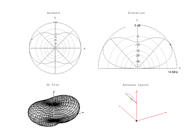
Directivity is a rough measure of an antenna. A more accurate measure is a radiation pattern plot. The radiation pattern plot is a graphical representation of intensity of radiation with respect to position throughout space. A radiation pattern plot may be a 3D plot or a pair of 2D plots. In the case where two 2D plots are used, one of the plots is an azimuth plot and the other is an elevation plot. The azimuth plot shows a horizontal slice of the 3D radiation pattern, parallel to the xy plane. The elevation plot shows a vertical slice, perpendicular to the xy plane. Most radiation pattern plots, including all shown in this text, are labeled by the amplitude of the electric field [15] [56]. However, occasionally they are labeled by the amplitude of the power instead. The radiation pattern of an antenna is quite different in the near field, at a distance less than about a wavelength, and in the far field, with distances much greater than a wavelength. Radiation pattern plots illustrate the far field behavior only.
Figure \(\PageIndex{1}\) shows the radiation pattern plot for a half-wave dipole antenna in free space, and it was plotted using the software EZNEC [56]. The acronym NEC stands for Numerical Electromagnetics Code. The figure in the upper left is the azimuth plot, the figure in the upper right is the elevation plot, the figure in the lower left is a 3D radiation pattern plot, and the figure in the lower right is the antenna layout.
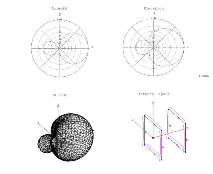
Figure \(\PageIndex{2}\) shows the radiation pattern plots for a 15-meter quad antenna. Distinct lobes and nulls are apparent.
Front to back ratio (\(\text{F/B ratio}\)) is a measure related to directivity that can be found from the azimuth radiation pattern plot. By definition, it is the ratio of the strength of the power radiated in the front to the back. Often, the front direction is chosen to be the direction of largest magnitude in the radiation pattern plot, and the back direction is the opposite direction. \(\text{F/B ratio}\) can be specified either on a log scale in units of \(\text{dB}\) or on a linear scale which is unitless. It can also be defined either as a ratio of the strength of the electric field intensities or as a ratio of the strengths of the powers, but most often power is used.
\[\text{F/B ratio} = \left[\frac{P_{front}}{P_{back}}\right]_{dB} = 10\log_{10}\left[\frac{P_{front}}{P_{back}}\right]_{lin} = 20\log_{10}\left[\frac{|\overrightarrow{E}_{front}|}{|\overrightarrow{E}_{back}|}\right]_{lin} \nonumber \]
\[\text{F/B ratio} = \left[\frac{P_{front}}{P_{back}}\right]_{dB} = 2\left[\frac{|\overrightarrow{E}_{front}|}{|\overrightarrow{E}_{back}|}\right]_{dB} \nonumber \]
The \(\text{F/B ratio}\) for the example of Fig. \(\PageIndex{2}\) can be calculated from the azimuth plot. The strength of the field in front direction is \(9 \text{dB}\) stronger than the strength of the field in the back direction.
\[\left[\frac{|\overrightarrow{E}_{front}|}{|\overrightarrow{E}_{back}|}\right]_{dB} = 9 \text{dB} \nonumber \]
From this information, we can calculate the strength of the field in the front direction to the strength of the field on a linear scale.
\[\left[\frac{|\overrightarrow{E}_{front}|}{|\overrightarrow{E}_{back}|}\right]_{dB} = 10\log_{10}\left[\frac{|\overrightarrow{E}_{front}|}{|\overrightarrow{E}_{back}|}\right]_{lin} \nonumber \]
\[\left[\frac{|\overrightarrow{E}_{front}|}{|\overrightarrow{E}_{back}|}\right]_{lin} = 10^{\frac{1}{10} \cdot \left[\frac{|\overrightarrow{E}_{front}|}{|\overrightarrow{E}_{back}|}\right]_{dB}} \nonumber \]
\[\left[\frac{|\overrightarrow{E}_{front}|}{|\overrightarrow{E}_{back}|}\right]_{lin} = 10^{\frac{9}{10}} = 7.94 \nonumber \]
If this antenna is being used as a transmitter, signal in the front direction is 7.9 times as strong as the signal in the back direction. The front to back ratio specifies the power ratio, and for this antenna, it is \(18 \text{dB}\).
\[\text{F/B ratio} = \left[\frac{P_{front}}{P_{back}}\right]_{dB} = 2\left[\frac{|\overrightarrow{E}_{front}|}{|\overrightarrow{E}_{back}|}\right]_{dB} = 18 \text{dB} \nonumber \]
When selecting an antenna, many decisions related to the antenna directivity are needed. A particular application may require an isotropic or a directional antenna. If a directional antenna is needed, the magnitude of the directivity must be decided. Additionally, the orientation of the antenna must be decided so that nodes and nulls are in the appropriate directions. Both the azimuth angle and the elevation angle of the nodes and nulls should be considered [50, p. 22-1].
Electromagnetic Polarization
The electromagnetic wave emanating from a transmitting antenna is described by an electric field \(\overrightarrow{E}\) and a magnetic field \(\overrightarrow{H}\). The wave necessarily has both an electric field and a magnetic field because, according to Maxwell's equations, time varying electric fields induce time varying magnetic fields, and time varying magnetic fields induce electric fields. At any point in space and at any time, the direction of the electric field, the direction of the magnetic field, and the direction of propagation of the wave are all mutually perpendicular. More specifically,
\[ \left( \text{Direction of } \overrightarrow{E} \right) \times \left( \text{Direction of } \overrightarrow{H} \right) = ( \text{Direction of propogation} ). \nonumber \]
An electromagnetic wave which varies with position in the same way that it varies with time is called a plane wave because planar wavefronts propagate at constant velocity in a given direction. For example, a sinusoidal plane wave which travels in the positive \(\hat{a}_z\) direction is described by
\[\overrightarrow{E} = E_0\cos(10^6t - 300z) \hat{a}_x . \nonumber \]
For this plane wave, \(\overrightarrow{E}\) is directed along \(\hat{a}_x\), \(\overrightarrow{H}\) is directed along \(\hat{a}_y\), and the wave propagates in the \(\hat{a}_z\) direction. As another example, consider the plane wave described by
\[\overrightarrow{E} = E_0\cos(10^6t - 300z) \left( \frac{\hat{a}_x + \hat{a}_y}{\sqrt{2}} \right) . \nonumber \]
For this plane wave, the direction of \(\overrightarrow{E}\) is \(45^{\circ}\) from the \(\hat{a}_x\) axis, the direction of \(\overrightarrow{H}\) is \(45^{\circ}\) from the \(\hat{a}_y\) axis, and again it propagates in the \(\hat{a}_z\) direction. Both of these electric fields describe sinusoidal plane waves because the electric field varies with position as it does with time, sinusoidally in both cases.
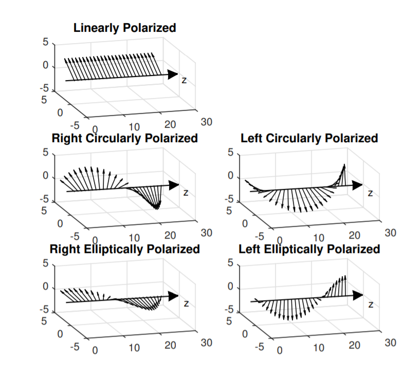
We can classify plane waves by their electromagnetic polarization. Plane waves can be classified as linearly polarized, left circularly polarized, right circularly polarized, left elliptically polarized, or right elliptically polarized. In a previous chapter, we encountered the distinctly different idea of material polarization. Appendix C discusses overloaded terminology including the term polarization.
Both of the electromagnetic waves described by Equation 4.4.13 and by Equation 4.4.14 are linearly polarized. In both cases, the direction of the electric field remains constant as the wave propagates with respect to both position and time. If the direction of the electric field rotates uniformly around the axis formed by the direction of propagation, the wave is called circularly polarized. If the direction of the electric field rotates nonuniformly, the wave is called elliptically polarized. For circularly polarized waves, the projection of the wave on a plane perpendicular to the axis formed by the direction of propagation is circular. For elliptical waves, the projection is elliptical. To determine if the polarization is left or right, point your right thumb in the direction of propagation, and compare the rotation of the electric field to the rotation of your fingers. If the rotation is along the direction of the fingers of your right hand, the wave is right polarized. Otherwise, it is left polarized. For example, the wave described by
\[\overrightarrow{E} =E_0\cos(10^6t - 300z) \frac{\hat{a}_x}{\sqrt{2}} + E_0\sin(10^6t - 300z) \frac{\hat{a}_y}{\sqrt{2}} \nonumber \]
is right circularly polarized. As another example, the wave
\[\overrightarrow{E} =E_0\cos(10^6t - 300z) \frac{\hat{a}_x}{2} + E_0\sin(10^6t - 300z) \frac{\hat{a}_y \sqrt{3}}{\sqrt{2}} \nonumber \]
is right elliptically polarized. The wave
\[\overrightarrow{E} =E_0\cos(10^6t - 300z) \frac{\hat{a}_x}{\sqrt{2}} - E_0\sin(10^6t - 300z) \frac{\hat{a}_y}{\sqrt{2}} \nonumber \]
is left circularly polarized. These definitions are illustrated in the Fig. \(\PageIndex{3}\).
What does electromagnetic polarization have to do with antennas? Antennas may be designed to transmit linearly, circularly, or elliptically polarized signals. Antennas designed to transmit or receive circularly polarized signals often contain wires that coil in the corresponding direction around an axis. If a signal is transmitted with an antenna designed to transmit linearly polarized waves, the best antenna to use as a receiver will be one that is also designed for linearly polarized waves. The signal can be detected by an antenna designed for signal of a different electromagnetic polarization, but the received signal will be noisier or weaker. Similarly, if a signal is transmitted with an antenna designed for right circular polarization, the best receiving antenna to use will be one also designed for right circular polarization.
Other Antenna Considerations
Antennas are made from good conductors. In Chapters 2 and 3, we saw that the materials that make up many energy conversion devices strongly influence the behavior. While the conductivity of conductors vary, overall the material that an antenna is made from does not significantly affect its behavior. In addition to bandwidth, impedance, directivity, and electromagnetic polarization, other factors, such as size, shape and configuration, distinguish one antenna from another. Mechanical factors should be considered too. An ideal antenna may be one that is easy to construct or mount in the desired location, is portable, or requires little maintenance [50]. If an antenna is to be mounted outside, the antenna should be able to withstand snow, wind, ice, and other extreme weather [50]. While Maxwell's equations are useful for predicting the radiation pattern of an antenna, they do not provide information about these other factors.
There is no perfect antenna. In one case, the best antenna may be a Yagi which is very directional and designed to operate within a narrow frequency band. In another application, the best antenna may be mechanically strong and mounted in a way to withstand extreme wind [50, p. 17-29]. In another case, the best antenna may be portable and easy to set up by one person regardless of its radiation pattern [50, p. 21-26]. In another case, the best antenna may be a wire of an arbitrary length hanging from a tree because it was the easiest and quickest to construct. As with any branch of engineering, antenna design involves trade offs. For example, the best antenna to detect an \(800 \text{ MHz}\) linearly polarized signal is an antenna that is designed to detect \(800 \text{ MHz}\) signals, is designed to detect linearly polarized signals, is oriented in the proper direction, and has an impedance matched to the impedance of the transmission line used. The signal can still be detected using an antenna designed for a different frequency, designed for a different electromagnetic polarization, improperly directed, or with mismatched impedance. However, in all of these cases, a less intense signal will be received.