1.8: Two Port Networks

So far, we have dealt with a number of networks which may be said to be one port or single-terminalpair circuits. That is, the important action occurs at a single terminal pair, and is characterized by an impedance and by either a open circuit voltage or a short circuit current, thus forming either a Thevenin or Norton equivalent circuit. A second, and for us very important, class of electrical network has two (or sometimes more) terminal pairs. We will consider formally here the two port network, illustrated schematically in Figure 21.

There are a number of ways of characterizing this type of network. For the time being, consider that it is passive, so that there is no output without some input and there are no dependent sources.

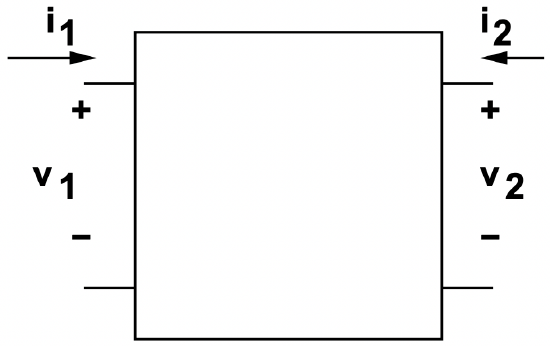Figure 21: Two-Port Network

Then we may characterize the network in terms of the currents at its terminals in terms of the voltages, or, conversely, we may describe the voltages in terms of the currents at the terminals. These two ways of describing the network are said to be the admittance or impedance parameters. These may be written in the following way:

The impedance parameter point of view would yield, for a resistive network, the following relationship between voltages and currents:

\[\ \left[\begin{array}{c}
v_{1} \\
v_{2}
\end{array}\right]=\left[\begin{array}{cc}
R_{11} & R_{12} \\
R_{21} & R_{22}
\end{array}\right]\left[\begin{array}{c}
i_{1} \\
i_{2}\label{14}
\end{array}\right] \nonumber \]

Similarly, the admittance parameter point of view would yield a similar relationship:

\[\ \left[\begin{array}{c}
i_{1} \\
i_{2}
\end{array}\right]=\left[\begin{array}{ll}
G_{11} & G_{12} \\
G_{21} & G_{22}
\end{array}\right]\left[\begin{array}{l}
v_{1} \\
v_{2}\label{15}
\end{array}\right] \nonumber \]

These two relationships are, of course, the inverses of each other. That is:

\[\ \left[\begin{array}{ll}
G_{11} & G_{12} \\
G_{21} & G_{22}
\end{array}\right]=\left[\begin{array}{cc}
R_{11} & R_{12} \\
R_{21} & R_{22}
\end{array}\right]^{-1}\label{16} \]

If the networks are linear and passive (i.e. there are no dependent sources inside), they also exhibit the property of reciprocity. In a reciprocal network, the transfer impedance or transfer admittance is the same in both directions. That is:

\(\ \begin{array}{l}
R_{12}=R_{21} \\
G_{12}=G_{21}
\end{array}\label{17}\)

It is often useful to express two- port networks in terms of T or Π networks, shown in Figures 22 and 23.

Sometimes it is useful to cascade two-port networks, as is shown in Figure 24. The resulting combination is itself a two-port. Suppose we have a pair of networks characterized by impedance parameters:

\(\ \left[\begin{array}{c}
v_{1} \\
v_{2}
\end{array}\right]=\left[\begin{array}{cc}
R_{11} & R_{12} \\
R_{12} & R_{22}
\end{array}\right]\left[\begin{array}{c}
i_{1} \\
i_{2}
\end{array}\right]\)

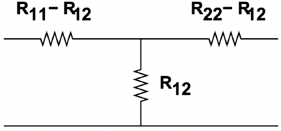Figure 22: T- Equivalent Network

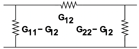Figure 23: Π-Equivalent Network

\(\ \left[\begin{array}{l}
v_{3} \\
v_{4}
\end{array}\right]=\left[\begin{array}{ll}
R_{33} & R_{34} \\
R_{34} & R_{44}
\end{array}\right]\left[\begin{array}{c}
i_{3} \\
i_{4}
\end{array}\right]\)

By noting that \(\ v_{2}=v_{3}\) and \(\ i_{3}=-i_{2}\), it is possible to show, with a little manipulation, that:

\(\ \left[\begin{array}{c}
v_{1} \\
v_{4}
\end{array}\right]=\left[\begin{array}{ll}
R_{11}^{\prime} & R_{14} \\
R_{14} & R_{44}^{\prime}
\end{array}\right]\left[\begin{array}{c}
i_{1} \\
i_{4}
\end{array}\right]\)

where

\(\ \begin{array}{c}
R_{11}^{\prime}=R_{11}-\frac{R_{12}^{2}}{R_{22}+R_{33}} \\
R_{44}^{\prime}=R_{44}-\frac{R_{34}^{2}}{R_{22}+R_{33}} \\
R_{14}=\frac{R_{12} R_{34}}{R_{22}+R_{33}}
\end{array}\)