1.9: Inductive and Capacitive Circuit Elements

So far, we have dealt with circuit elements which have no memory and which, therefore, are characterized by instantaneous behavior. The expressions which are used to calculate what these elements are doing are algebraic (and for most elements are linear too). As it turns out, much of the circuitry we will be studying can be so characterized, with complex parameters.

However, we take a quick diversion to discuss briefly the transient behavior of circuits containing capacitors and inductors.

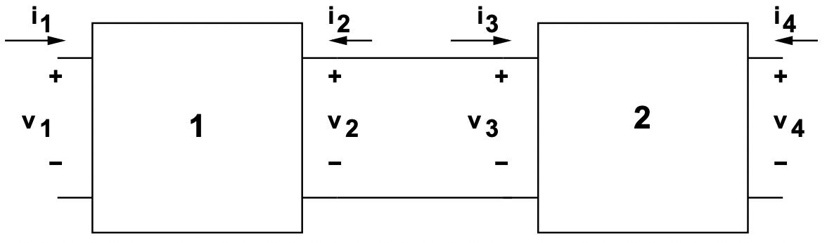Figure 24: Cascade of Two-Port Networks

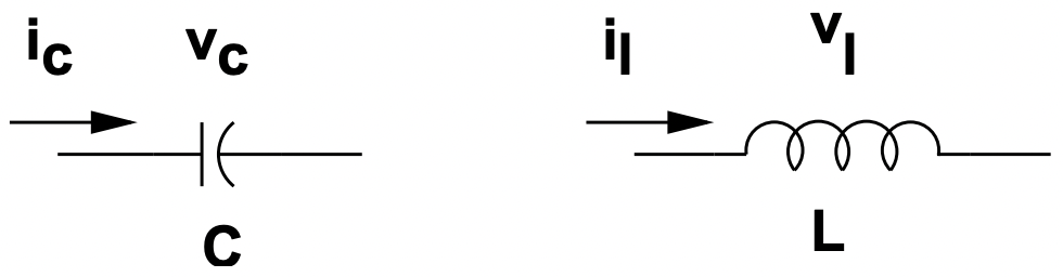Figure 25: Capacitance and Inductance

Symbols for capacitive and inductive circuit elements are shown in Figure 25. They are characterized by the relationships between voltage and current:

\[\ i_{c}=C \frac{d v_{c}}{d t} \quad\quad\quad v_{\ell}=L \frac{d i_{\ell}}{d t}\label{18} \]

Note that, while these elements are linear, since time derivatives are involved in their characterization, expressions describing their behavior in networks will become ordinary differential equations

Simple Case: R-C

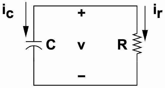Figure 26: Simple Case: R-C

Figure 26 shows a simple connection of a resistance and a capacitance. This circuit has only two nodes, so there is a single voltage v across both elements. The two elements produce the constraints:

\(\ \begin{aligned}
i_{r} &=\frac{v}{R} \\
i_{c} &=\frac{d v}{d t}
\end{aligned}\)

and, since \(\ i_{r}=-i_{c}\),

\(\ \frac{d v}{d t}+\frac{1}{R C} v=0\)

Now, we know that this sort of first-order, linear equation is solved by:

\(\ v \sim e^{-\frac{t}{R C}}\)

(To confirm this, just substitute the exponential into the differential equation.) Then, if we have some initial condition, say \(\ v(t=0)=V_{0}\), then

\(\ v=V_{0} e^{-\frac{t}{R C}}\)

This was a trivial case, since we don’t describe how that initial condition might have taken place. But consider a closely related problem, illustrated in Figure 27.

Simple Case with Drive

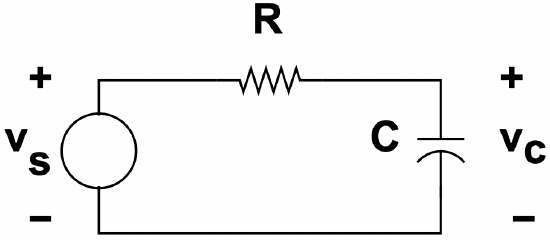Figure 27: RC Circuit with Drive

The analysis of this circuit is accomplished by noting that it contains a single loop, and adding up the voltages around the loop we find:

\(\ R C \frac{d v_{c}}{d t}+v_{c}=v_{s}\)

Now, assume that the voltage source is a step:

\(\ v_{s}=V_{s} u_{-1}(t)\)

We should define the step function with some care, since it is of quite a lot of use. The step is one of a hierarchy of singularity functions. It is defined as:

\[\ u_{-1}(t)=\left\{\begin{array}{ll}
0 & t<0 \\
1 & t>0
\end{array}\right. \label{19} \]

Now, remembering that differential equations have particular and homogeneous solutions, and that for \(\ t>0\) a particular solution which solves the differential equation is:

\(\ v_{c p}=V\)

Of course this does not satisfy the initial condition which is that the capacitance be uncharged: \(\ v_{c}(t=0+)=0\). Again, remember that the whole solution is the sum of the particular and a homogeneous solution, and that the homogeneous solution is the un-driven case. To satisfy the initial condition, the homogeneous solution must be:

\(\ c_{c h}=-V e^{-\frac{t}{R C}}\)

So that the total solution is simply:

\(\ v_{c}=V\left(1-e^{-\frac{t}{R C}}\right)\)

Next, suppose \(\ v_{s}=u_{-1}(t) V \cos \omega t\). We know the homogeneous solution must be of the same form, but the particular solution is a bit more complicated. In later chapters we will learn how to make the process of extracting the particular solution easier, but for the time being, let’s assume that with a sinusoidal drive we will get a sinusoidal response of the same frequency. Thus we will guess

\(\ v_{c p}=V_{c p} \cos (\omega t-\phi)\)

The time derivative is

\(\ \frac{d v_{c p}}{d t}=\omega V_{c p} \sin (\omega t-\phi)\)

so that we can find an algebraic equation for the particular solution:

\(\ V \cos \omega t=V_{c p}(\cos (\omega t-\phi)+\omega R C \sin (\omega t-\phi))\)

Note the trigonometric identities:

\(\ \begin{aligned}
\cos (\omega t-\phi) &=\cos \phi \cos \omega t+\sin \phi \sin \omega t \\
\sin (\omega t-\phi) &=-\sin \phi \cos \omega t+\cos \phi \sin \omega t
\end{aligned}\)

Since the sine and cosine terms are orthogonal, we can equate coefficients of sine and cosine to get:

\(\ \begin{aligned}
V &=V_{c p}[\cos \phi+\omega R C \sin \phi] \\
0 &=V_{c p}[\sin \phi+\omega R C \cos \phi]
\end{aligned}\)

The second of these can be solved for the phase angle:

\(\ \phi=\tan ^{-1} \omega R C\)

and squaring both equations and adding:

\(\ V^{2}=V_{c p}^{2}\left(1+(\omega R C)^{2}\right)\)

so that the particular solution is:

\(\ v_{c p}=\frac{V}{\sqrt{1+(\omega R C)^{2}}} \cos (\omega t-\phi)\)

Finally, if the capacitor is initially uncharged \(\ \left(v_{c}(t=0+)=0\right)\), we can add in the homogeneous solution (we already know the form of this), and find the total solution to be:

\(\ v_{c} p=\frac{V}{\sqrt{1+(\omega R C)^{2}}}\left[\cos (\omega t-\phi)-\cos \phi e^{-\frac{t}{R C}}\right]\)

This is shown in Figure 28

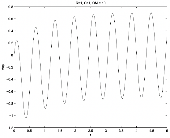Figure 28: Output Voltage for RC Example

Second-Order System Example

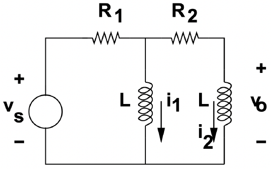Figure 29: Two-Inductor Circuit

Figure 29 shows a network with two inductances and two resistances. Assume that this is driven by a voltage step: \(\ v_{s}=V_{s} u_{-1}(t)\). Note that, with two inductances, we will require two initial conditions to complete the solution.

The steady state (particular) solution is \(\ v_{o}=0\). There will, of course, be current flowing in each of the inductances, but if excitation is constant there will be no time derivative of current so that voltage across each of the inductances will eventually fall to zero.

The initial conditions may be found by inspection. Right after \(\ t=0\) (note we use \(\ t=0+\) for this), output voltage must be:

\(\ v_{o}(t=0+)=V_{s}\)

This must be so since current cannot be made to flow instantaneously in either inductance, so that there is no current in either resistance.

The second initial condition is the rate of change of voltage right after the instant of the voltage step. To find this, note that output voltage is equal to the source voltage minus the voltage drops across each of the two resistances.

\(\ v_{o}=v_{s}-R_{2} i_{2}-R_{1}\left(i_{1}+i_{2}\right)\)

If we differentiate this with respect to time and note that the time derivative of a constant (after the step the input voltage is constant) is zero:

\(\ \frac{d v_{o}}{d t}(t=0+)=-\left(R_{1}+R_{2}\right) \frac{d i_{2}}{d t}-R_{1} \frac{d i_{1}}{d t}\)

Now, since right after the instant of the step both inductances have the source voltage \(\ V_{s}\) across them:

\(\ \left.\frac{d i_{1}}{d t}\right|_{t=0+}=\left.\frac{d i_{2}}{d t}\right|_{t=0+}=\frac{V_{s}}{L}\)

the rate of change of voltage at \(\ t=0+\) is:

\(\ \left.\frac{d v_{o}}{d t}\right|_{t=0+}=-\frac{2 R_{1}+R_{2}}{L} V_{s}\)

Now, we can find the homogeneous solution using the loop method. Setting the source to zero, assume a current \(\ i_{a}\) in the left-hand loop and \(\ i_{b}\) in the right-hand loop. KVL around these two loops yields:

\(\ \begin{array}{c}
R_{1} i_{a}+L \frac{d}{d t}\left(i_{a}-i_{b}\right)=0 \\
R_{2} i_{b}+2 L \frac{d i_{b}}{d t}-L \frac{d i_{a}}{d t}=0
\end{array}\)

With a little manipulation, these become:

\(\ \begin{array}{c}
L \frac{d i_{a}}{d t}+2 R_{1} i_{a}+R_{2} i_{b}=0 \\
L \frac{d i_{b}}{d t}+R_{1} i_{a}+R_{2} i_{b}=0
\end{array}\)

Assume that solutions are of the form \(\ I e^{s t}\), and this set of simultaneous equations becomes:

\(\ \left[\begin{array}{cc}
\left(s L+2 R_{1}\right) & R_{2} \\
R_{1} & \left(s L+R_{2}\right)
\end{array}\right]\left[\begin{array}{c}
I_{a} \\
I_{b}
\end{array}\right]=\left[\begin{array}{l}
0 \\
0
\end{array}\right]\)

We need to solve this for s (to find values of s for which this set is true, and that is simply the solution of the “characteristic equation”

\(\ \left(s L+2 R_{1}\right)\left(s L+R_{2}\right)-R_{1} R_{2}=0\)

which is the same as:

\(\ s^{2}+\frac{2 R_{1}+R_{2}}{L} s+\frac{R_{1}}{L} \frac{R_{2}}{L}=0\)

Now, for the sake of “nice numbers”, assume that R1 = 2R, R2 = 3R. The characteristic equation is:

\(\ s^{2}+7 \frac{R}{L} s+6\left(\frac{R}{L}\right)^{2}=0\)

which factors nicely into \(\ \left(s+\frac{R}{L}\right)\left(s+6 \frac{R}{L}\right)=0\\), or the two values of s are \(\ s=-\frac{R}{L}\) and \(\ s=-6 \frac{R}{L}\).

Since the particular solution to this one is zero, we have a total solution which is:

\(\ v_{o}=A e^{-\frac{R}{L} t}+B e^{-6 \frac{R}{L} t}\)

The initial conditions are:

\(\ \begin{aligned}
\left.v_{o}\right|_{t=0+}=A+B &=V_{s} \\
\left.\frac{d v_{o}}{d t}\right|_{t=0+}=-\frac{R}{L}(A+6 B) &=-7 \frac{R}{L} V_{s}
\end{aligned}\)

The solution to that pair of expressions is:

\(\ A=-\frac{V_{s}}{5} \quad\quad B=\frac{6 V_{s}}{5}\)

and this is shown in Figure 30.

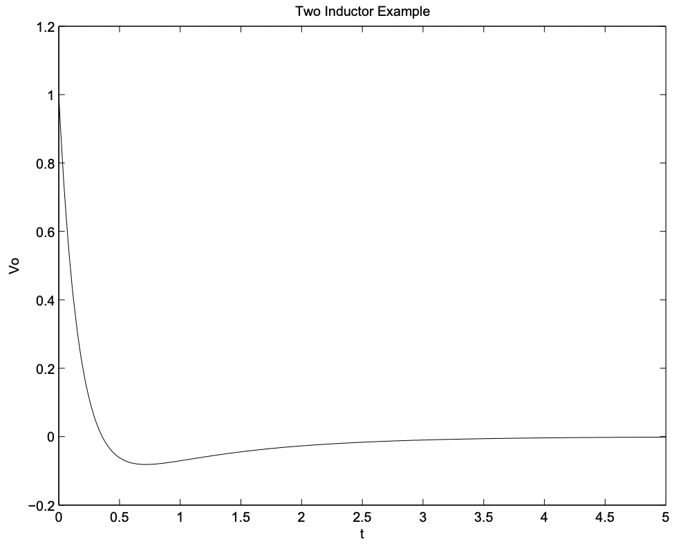Figure 30: Output Voltage for Two Inductor Example