2.1: Transmission Lines

A transmission line is really a long, continuous thing. It has inductance which is really inductance per unit length multiplied by the line length, but it also has a continuous capacitance. We might attempt to represent a long transmission line as a series of relatively ’short’ sections each represented by an inductance and a capacitance. These ’lumped parameter’ models for lines are actually used in many system studies, particularly in physical analog models called ’Transmission System Simulators’. (We built one of these at MIT in the 1970’s). After the next section you might contemplate the definition of ’short’ for our purposes here, but generally each lumped parameter capacitance and resistance pair would represent a few to a few tens of miles.

Telegrapher’s Equations

Peering at the model presented in Figure 22, one might divine that a proper representation of voltage and current, both of which are functions of time and distance along the line, might be:

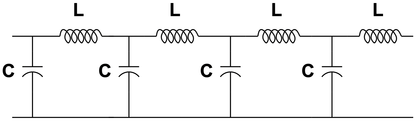Figure 22: Transmission Line Lumped Parameter Model

\(\ \begin{array}{l}
\frac{\partial v}{\partial x}=-L_{l} \frac{\partial i}{\partial t} \\
\frac{\partial i}{\partial x}=-C_{l} \frac{\partial v}{\partial t}
\end{array}\)

These are known as the “Telegrapher’s Equations” and represent the fact that inductance presents voltage drop along the line in proportion to rate of change of current and that capacitance presents a change in current along the line in proportion to rate of change of voltage.

It is not difficult to eliminate either voltage or current from these to produce a wave equation. For example, take the cross-derivatives and substitute the second of these equations into the first to get:

\(\ \frac{\partial^{2} v}{\partial x^{2}}=L_{l} C_{l} \frac{\partial^{2} v}{\partial t^{2}}\)

Now: this equation is solved by arbitrary functions which are of the form:

\(\ v(x, t)=v(x \pm u t)\)

where the wave velocity is:

\(\ u=\frac{1}{\sqrt{L_{l} C_{l}}}\)

So now we can see that the voltage on the line is the sum of some waveform going in the ’positive’ direction and something else going in the ’negative’ direction:

\(\ v(x, t)=v_{+}(x-u t)+v_{-}(x+u t)\)

The same will be true of current, and substituting back into either of the telegrapher’s equations yields:

\(\ i(x, t)=\frac{1}{L_{l} u}\left(v_{+}(x-u t)-v_{-}(x+u t)\right)\)

the product of inductance times wave velocity has the units of impedance:

\(\ L_{l} u=\sqrt{\frac{L_{l}}{C_{l}}}=Z_{0}\)

This is often referred to as the ’characteristic impedance’ of the transmission line. This is also a commonly used term: transmission cables are often referred to by their characteristic impedances. For coaxial wires 50 to 72 ohms are common values. For high tension transmission lines somewhat higher values are to be expected.

Surges on Transmission Lines

Consider the situation shown in Figure 23. Here the left-hand end of the line is driven by a current source with a pulse (illustrated is a square pulse). This is actually not too far from the situation that transmission lines experience with lightning, which is usually representable as a current source, typically of magnitude between 20 and 100 kA and duration of about 1µS. (Actually, it is not a square pulse but that is not important here).

What will happen, if the pulse is short enough, is that it will launch a traveling wave in which \(\ v_{+}=Z_{0} i_{+}\) and \(\ i_{+}\) is the current that was imposed. When this pulse reaches the far, or load end of the line, we have the situation in which at that point:

\(\ \begin{aligned}
v(t) &=v_{+}+v_{-} \\
i(t) &=\frac{v_{+}}{Z_{0}}-\frac{V_{-}}{Z_{0}}
\end{aligned}\)

and, of coures, \(\ v=R i\).

The ’reflected’, or negative going wave will have magnitude:

\(\ v_{-}=v_{+} \frac{\frac{R}{Z_{0}}-1}{\frac{R}{Z_{0}}+1}\)

In the extreme case of an open circuit, the magnitude of the voltage pulse at the end of the transmission line is exactly twice that of the propagating pulse. In the case of a short circuit, of course, the magnitude of the voltage is zero, the current in the short is double the current of the pulse itself, and the pulse is reflected, but going in the reverse direction with a polarity the opposite of the forward-going pulse. This is illustrated in cartoon form in Figure 23.

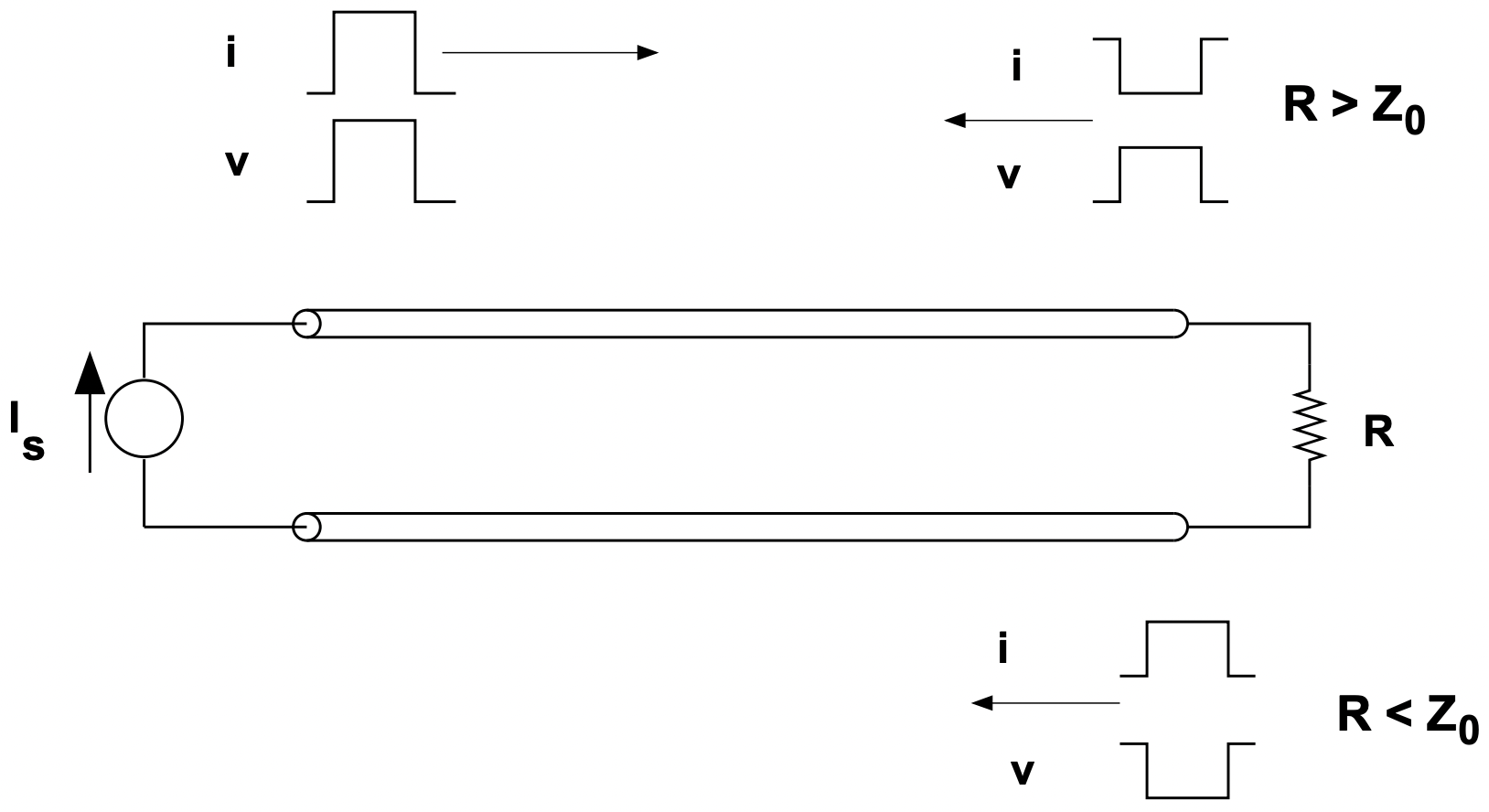Figure 23: Pulse Propagation on a Transmission Line

Sinusoidal Steady State

Now, consider a transmission line operating in the sinusoidal steady state. As suggested by Figure 24, it is driven by a voltage source at one end and is loaded by a resistive load at the other. Consistent with the voltage and currents that we know can exist on such a line, we know they will be of this form:

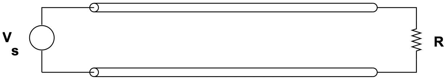Figure 24: Transmission Line in Simple Configuration

\(\ \begin{aligned}
v(x, t) &=\operatorname{Re}\left\{\underline{V}_{+} e^{j(\omega t-k x)}+\underline{V}_{-} e^{j(\omega t+k x)}\right\} \\
i(x, t) &=\operatorname{Re}\left\{\frac{V_{+}}{Z_{0}} e^{j(\omega t-k x)}-\frac{V}{Z_{0}} e^{j(\omega t+k x)}\right\}
\end{aligned}\)

Where the phase velocity is \(\ u=\frac{\omega}{k}=\frac{1}{\sqrt{L_{l} C_{l}}}\).

At the termination end of the line, at \(\ x=\ell\)

\(\ \begin{equation}
R=\frac{\underline{V}}{\underline{I}}=Z_{0} \frac{\underline{V}_{+} e^{-j k \ell}+\underline{V}_{-} e^{j k \ell}}{\underline{V}_{+} e^{-j k \ell}-\underline{V}_{-} e^{j k \ell}}
\end{equation}\)

This may be solved for the ratio of ’reverse’ to ’forward’ amplitude:

\(\ \begin{equation}
\underline{V}_{-}=\underline{V}_{+} e^{-2 j k \ell} \frac{\frac{R}{Z_{0}}-1}{\frac{R}{Z_{0}}+1}
\end{equation}\)

Since at the ’sending’ end:

\(\ \begin{equation}
V_{s}=\underline{V}_{+}+\underline{V}_{-}
\end{equation}\)

With a little manipulation it can be determined that

\(\ \underline{V}_{r}=V_{s} \frac{e^{-j k \ell}\left[\left(\frac{R}{Z_{0}}+1\right)+\left(\frac{R}{Z_{0}}-1\right)\right]}{\left(\frac{R}{Z_{0}}+1\right)+e^{-2 j k \ell}\left(\frac{R}{Z_{0}}-1\right)}\)

Further manipulation yields:

\(\ \underline{V}_{r}=V_{s} \frac{\frac{R}{Z_{0}}}{\frac{R}{Z_{0}} \cos k \ell+j \sin k \ell}\)

This might be made a bit more comprehensible when turned into a magnitude:

\(\ \left|\frac{V_{r}}{V_{s}}\right|=\frac{\frac{R}{Z_{0}}}{\sqrt{\left(\frac{R}{Z_{0}} \cos k \ell\right)^{2}+(\sin k \ell)^{2}}}\)

If the line is loaded with a resistance equivalent to the ’surge impedance’ (so-called ’surge impedance loading’, the receiving end voltage is the same as the sending end voltage. If it is more heavily loaded, the receiving end voltage is less than the sending end and if it is less heavily loaded the receiving end voltage is greater.