2.4: Impedance

Because it is so easy to differentiate a complex exponential time signal, such a way of representing time signals has real advantages in electric circuits with all kinds of linear elements. In Section 1 of these notes, we introduced the linear resistance element, in which voltage and current are linearly related. We must now consider two other elements, inductances and capacitances. The inductance produces a relationship between voltage and current which is:

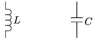Figure 4: Inductance and Capacitance Elements

\[\ v_{L}=L \frac{d i_{L}}{d t}\label{35} \]

If voltage and current are sinusoidal functions of time:

\(\ \begin{aligned}
v &=\underline{V} e^{j \omega t}+\underline{V}^{*} e^{-j \omega t} \\
i &=\underline{I} e^{j \omega t}+\underline{I}^{*} e^{-j \omega t}
\end{aligned}\)

Then the relationship between voltage and current is given simply by:

\[\ \underline{V}=j \omega L \underline{I}\label{36} \]

This is a particularly simple form, and as can be seen is directly analogous to resistance. We can generalize our view of resistance to complex impedance (or simply impedance), in which inductances have impedance which is:

\[\ \underline{Z}_{L}=j \omega L\label{37} \]

The capacitance element is similarly defined. A capacitance has a voltage-current relationship:

\[\ i=C \frac{d v_{C}}{d t}\label{38} \]

Thus the impedance of a capacitance is:

\[\ \underline{Z}_{C}=\frac{1}{j \omega C}\label{39} \]

The extension to resistive network behavior is now obvious. For problems in sinusoidal steady state, in which all excitations are sinusoidal, we may use all of the tricks of linear, resistive network analysis. However, we use complex impedance in place of resistance.

The inverse of impedance is admittance:

\(\ \underline{Y}=\frac{1}{\underline{Z}}\)

Series and parallel combinations of admittances and impedances are, of course, just like those of conductances and resistances. For two elements in series or in parallel:

Series:

\[\ \underline{Z}=\underline{Z}_{1}+\underline{Z}_{2}\label{40} \]

\[\ \underline{Y}=\frac{\underline{Y}_{1} \underline{Y}_{2}}{\underline{Y}_{1}+\underline{Y}_{2}}\label{41} \]

Parallel:

\[\ \underline{Z}=\frac{\underline{Z}_{1} \underline{Z}_{2}}{\underline{Z}_{1}+\underline{Z}_{2}}\label{42} \]

\[\ \underline{Y}=\underline{Y}_{1}+\underline{Y}_{2}\label{43} \]

Example

Suppose we are to find the voltage \(\ v(t)\) in the network of Figure 5, in which \(\ i(t)=I \cos (\omega t)\). The excitation may be written as:

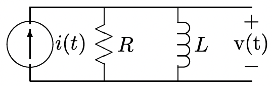Figure 5: Complex Impedance Network

\(\ i(t)=\frac{I}{2} e^{j \omega t}+\frac{I}{2} e^{-j \omega t}=\operatorname{Re}\left(I e^{j \omega t}\right)\)

Now, the complex impedance of the parallel combination of \(\ R\) and \(\ L\) is:

\(\ R \| j \omega L=\frac{R j \omega L}{R+j \omega L}\)

So that, if \(\ v(t)\) is represented by:

\(\ \begin{aligned}
v(t) &=\frac{V}{2} e^{j \omega t}+\frac{V}{2} e^{-j \omega t} \\
&=R e\left(\underline{V} e^{j \omega t}\right)
\end{aligned}\)

Then

\(\ \underline{V}=\frac{R j \omega L}{R+j \omega L} I\)

Now: the impedance \(\ \underline{Z}\) may be represented by a magnitude and phase angle:

\(\ \begin{aligned}
\underline{Z} &=|\underline{Z}| e^{j \phi} \\
|\underline{Z}| &=\frac{\omega L R}{\sqrt{(\omega L)^{2}+R^{2}}} \\
\phi &=\frac{\pi}{2}-\arctan \frac{\omega L}{R}
\end{aligned}\)

Then, using relations developed here, \(\ v(t)\) may be written as:

\(\ v(t)=\frac{\omega L I}{\sqrt{1+\left(\frac{\omega L}{R}\right)^{2}}} \cos (\omega t+\phi)\)

Note that this expression represents only the sinusoidal steady state solution, and therefore does not represent any starting transients.