2.5: System Functions and Frequency Response

Last updated
Save as PDF

Page ID: 55523

James Kirtley
Massachusetts Institute of Technology via MIT OpenCourseWare

\( \newcommand{\vecs}[1]{\overset { \scriptstyle \rightharpoonup} {\mathbf{#1}} } \) \( \newcommand{\vecd}[1]{\overset{-\!-\!\rightharpoonup}{\vphantom{a}\smash {#1}}} \)\(\newcommand{\id}{\mathrm{id}}\) \( \newcommand{\Span}{\mathrm{span}}\) \( \newcommand{\kernel}{\mathrm{null}\,}\) \( \newcommand{\range}{\mathrm{range}\,}\) \( \newcommand{\RealPart}{\mathrm{Re}}\) \( \newcommand{\ImaginaryPart}{\mathrm{Im}}\) \( \newcommand{\Argument}{\mathrm{Arg}}\) \( \newcommand{\norm}[1]{\| #1 \|}\) \( \newcommand{\inner}[2]{\langle #1, #2 \rangle}\) \( \newcommand{\Span}{\mathrm{span}}\) \(\newcommand{\id}{\mathrm{id}}\) \( \newcommand{\Span}{\mathrm{span}}\) \( \newcommand{\kernel}{\mathrm{null}\,}\) \( \newcommand{\range}{\mathrm{range}\,}\) \( \newcommand{\RealPart}{\mathrm{Re}}\) \( \newcommand{\ImaginaryPart}{\mathrm{Im}}\) \( \newcommand{\Argument}{\mathrm{Arg}}\) \( \newcommand{\norm}[1]{\| #1 \|}\) \( \newcommand{\inner}[2]{\langle #1, #2 \rangle}\) \( \newcommand{\Span}{\mathrm{span}}\)\(\newcommand{\AA}{\unicode[.8,0]{x212B}}\)

If we are interested in the behavior of a linear system such as the circuits we have been discussing, we often speak of the system function. This is the (usually complex) ratio between output and input of the system. System functions can express driving point behavior (impedance or its reciprocal, admittance) or transfer behavior. We speak of voltage or current transfer ratios and of transfer impedance (output voltage related to input current) and transfer admittance (output current related to input voltage).

The system function may be expressed in a number of ways, often as a Laplace Transform. Such is beyond the scope of this subject. However, it is important to understand one way of expressing linear system behavior, in the form of frequency response. The frequency response of a system is the complex number that relates output of the system to input as a function of frequency. Usually it is expressed as a pair of numbers, magnitude and phase angle. Thus

\[\ H(j \omega)=|H(j \omega)| e^{j \phi(j \omega)} \nonumber \]

Subjects in Signals and Systems or Network Theory often spend some time on how to obtain and plot the frequency response of a network in ways which are both useful and easy. For our purposes, a straightforward, perhaps even “brute force” approach will do. Consider, for example, the circuit shown in Figure 6.

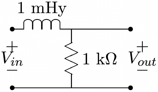
Screen Shot 2021-07-19 at 2.49.18 PM.png — Figure 6: Example Circuit for Frequency Response

This is just a voltage divider between an inductance and a resistance. We seek to find, and then plot, the transfer ratio \(\ V_{\text {out }} / V_{\text {in }}\) of this network. A very little analysis yields an expression for the transfer function, which is:

\[\ \dfrac{V_{\text {out }}(j \omega)}{V_{\text {in }}(j \omega)}=\dfrac{R}{R+j \omega L}=\dfrac{1}{1+j \omega \dfrac{L}{R}} \nonumber \]

The magnitude and angle of this function can be extracted in a number of ways. For the purpose of these notes, we have done the mathematics using MATLAB. The specific instructions for producing the frequency response plot are shown in Figure 7. Funamentally what is done is to compute the system function for a number of frequencies (note that we use a way of computing specific frequencies which produces a uniform spacing on a logarithmic scale, and then plotting the magnitude (also on a logarithmic scale) and angle of that system function against frequency.