2.6: Phasors

Phasors are not weapons. They are a handy geometric trick which help us understand the nature of sinusoidal steady state signals and systems. To start, consider the basis for complex exponential time notation, the function \(\ e^{j \omega t}\). At any instant of time, this is a complex number: at time \(\ t=0\) it is equal to 1, at time \(\ \omega t=\frac{\pi}{2}\) it is equal to \(\ j\), and so forth. We may describe this function as a vector, of length unity, rotating about the origin of the complex number plane, with angular velocity \(\ \omega\). It has, of course, both real and imaginary parts, which are just the projections of the vector onto the real and imaginary axes.

Now consider a sinusoidally varying signal \(\ x(t)\), which may be represented by:

\(\ x(t)=\frac{X}{2} e^{j \omega t}+\frac{X^{*}}{2} e^{-j \omega t}\)

This is the sum of two numbers, complex conjugates, which are, as functions of time, rotating in opposite directions in the complex plane. The sum of the two is, of course, real. This is the same time function as:

\[\ x(t)=\operatorname{Re}\left(\underline{X} e^{j \omega t}\right)\label{44} \]

where the real part operator \(\ {Re}(\cdot)\) simply takes the projection of the function on the real axis.

It might be helpful at this point to remember one of the features of complex arithmetic. Multiplication of two complex numbers results in a third complex number which has:

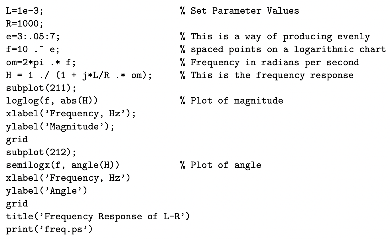Figure 7: MATLAB Program freq.m

1. a magnitude which is the product of the magnitudes of the two numbers begin multiplied and,
2. an angle which is the sum of the angles of the two numbers being multiplied.

Thus, multiplying a number by \(\ e^{j \omega t}\), which has a magnitude of unity and an angle which is increasing with time at the rate \(\ \omega\), simply has the effect of setting that number spinning around the origin of the complex plane.

It is therefore relatively easy to represent sinusoidally varying signals with just their complex amplitudes, understanding that they also include \(\ e^{j \omega t}\), which provides time variation. The complex amplitude includes not only the magnitude of the signal, but also a phase angle. Usually the phase angle by itself is of little use, and must be related to some time reference. That is, as we will see, it is the difference between phase angles that is important in most cases.

Impedances and admittances are also complex numbers, so that phasors can be used to visualize the relationship between voltages and currents in a network. The key here is that multiplication and division of complex numbers is the same as multiplication or division of magnitudes and addition or subtraction of angles.

Example

Consider the simple network shown in Figure 9, and suppose that the current source is sinusoidal:

\(\ i=\operatorname{Re}\left(\underline{I} e^{j \omega t}\right)\)

The impedance of the R-L combination is a complex number:

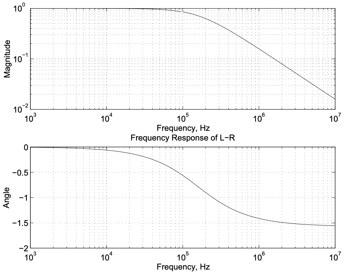Figure 8: Frequency Response

\(\ \underline{Z}=R+j \omega L=1+j 2\)

Now: the impedance may be represented in the complex plane as shown in Figure 10.

Voltage \(\ v\) is given by:

\(\ v=R e\left(\underline{V} e^{j \omega t}\right)\)

where:

\(\ \underline{V}=\underline{Z I}\)

Then the relationship between voltage and current is as shown in Figure 11. Note that the phase angle between voltage and current is the same as the phase angle of the impedance.

Note that KVL may be represented graphically in the fashion of Figure 12.