2.7: Energy and Power

For any terminal pair with voltage and current defined as shown in Figure 13, power flow into the element is:

\[\ p=v i\label{45} \]

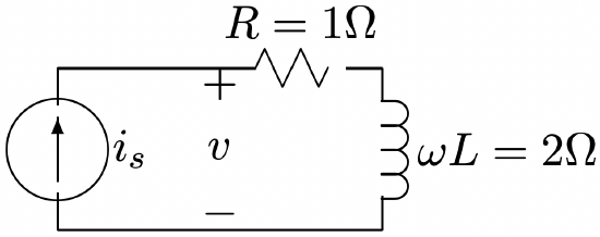Figure 9: Example Circuit

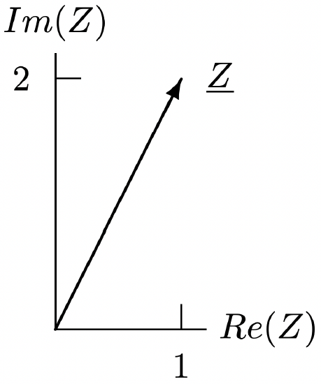Figure 10: Complex Impedance

Power is expressed in Watts (W), and one Watt is the product of one Volt and one Ampere. Energy transferred over an interval of time \(\ t_{0}\) to \(\ t_{1}\) is the integral of power:

\[\ w=\int_{t_{0}}^{t_{1}} v(t) i(t) d t\label{46} \]

Energy is expressed in Joules, and one Joule is one Watt- Second. A Joule is also a Newton-Meter (force times distance), and therefore a Watt is a Newton-Meter per Second.

Consider the behavior of the three types of linear, passive elements we have encountered:

• \[\ p=R i^{2}=\frac{v^{2}}{R}\label{47} \]

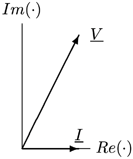  Figure 11: Voltage and Current

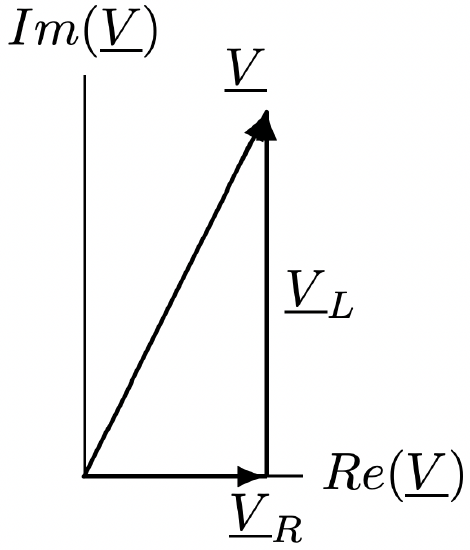  Figure 12: Components of Voltage

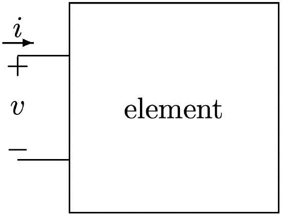  Figure 13: Definition for Power

• \[\ p=i L \frac{d i}{d t}=\frac{1}{2} L \frac{d i^{2}}{d t}\label{48} \]

  The quantity \(\ w_{L}=\frac{1}{2} L i^{2}\) may be interpreted as energy stored in the inductance, so that \(\ p=\frac{d w_{L}}{d t}\). We will need to refine this definition later, when we consider electromechanical interactions or nonlinear elements, but it will do for now.

• \[\ p=v C \frac{d v}{d t}=\frac{1}{2} C \frac{d v^{2}}{d t}\label{49} \]

  The quantity \(\ w_{C}=\frac{1}{2} C v^{2}\) may similarly be interpreted as energy stored in the capacitance.

  Next, consider the power input to each of these three elements under sinusoidal steady state conditions:

• Resistance: if \(\ i=I \cos (\omega t+\theta)\), then

  \[\ \begin{aligned}
  p &=R I^{2} \cos ^{2}(\omega t+\theta) \\
  &=\frac{R I^{2}}{2}[1+\cos 2(\omega t+\theta)]
  \end{aligned}\label{50} \]

  Thus, average power into the resistance is:

  \[\ P=\frac{1}{2} R I^{2}\label{51} \]

• Inductance: if \(\ i=I \cos (\omega t+\theta)\), then voltage is \(\ v=-\omega L I \sin (\omega t+\theta)\), and power is:

  \[\ \begin{aligned}
  p &=-\omega L I^{2} \cos (\omega t+\theta) \sin (\omega t+\theta) \\
  &=-\frac{\omega L I^{2}}{2} \sin 2(\omega t+\theta)
  \end{aligned}\label{52} \]

  Average power into the inductance is zero. Instantaneous energy stored in the inductance is

  \(\ w_{L}=\frac{1}{2} L I^{2} \cos ^{2}(\omega t+\theta)\)

  and that has an average value:

  \[\ <w_{L}>=\frac{1}{4} L I^{2}\label{53} \]

• \[\ p=-\frac{\omega C V^{2}}{2} \sin 2(\omega t+\phi)\label{54} \]

  which has zero time average. Energy stored in the capacitance is:

  \(\ w_{C}=\frac{1}{2} C V^{2} \cos ^{2}(\omega t+\phi)\)

  which has time average:

  \[\ <w_{C}>=\frac{1}{4} C V^{2}\label{55} \]

Now, consider power flow into a set of terminals in a situation in which both voltage and current are sinusoidal and have the same frequency, but possibly different phase angles:

\(\ \begin{aligned}
v(t) &=V \cos (\omega t+\phi) \\
i(t) &=I \sin (\omega t+\theta)
\end{aligned}\)

It is necessary to revert to the original form of complex notation, as in equation 19, to compute power.

\[\ v(t)=\frac{1}{2}\left[\underline{V} e^{j \omega t}+\underline{V}^{*} e^{-j \omega t}\right]\label{56} \]

\[\ i(t)=\frac{1}{2}\left[\underline{I} e^{j \omega t}+\underline{I}^{*} e^{-j \omega t}\right]\label{57} \]

Instantaneous power is the product of voltage and current:

\[\ p=\frac{1}{4}\left[\underline{V I}^{*}+\underline{V}^{*} \underline{I}+\underline{V I} e^{j 2 \omega t}+\underline{V}^{*} \underline{I}^{*} e^{-j 2 \omega t}\right]\label{58} \]

This is directly equivalent to:

\[\ p=\frac{1}{2} R e\left[\underline{V I}^{*}+\underline{V I} e^{j 2 \omega t}\right]\label{59} \]

This is, in turn, expressible as:

\[\ p=\frac{1}{2}|\underline{V} \| \underline{I}|[\cos (\phi-\theta)+\cos (2 \omega t+\phi+\theta)]\label{60} \]

From this, we extract “real power”, or time- average power:

\[\ P=\frac{1}{2} \operatorname{Re}\left[\underline{V I}^{*}\right]=\frac{1}{2}|\underline{V} \| \underline{I}| \cos (\phi-\theta)\label{61} \]

The ratio between real power and apparent power \(\ P_{a}=\frac{1}{2}|\underline{V} \| \underline{I}|\) is called the power factor, and is simply:

\[\ \text { power factor }=\cos \psi=\cos (\phi-\theta)\label{62} \]

The power factor angle \(\ \psi=\phi-\theta\) is the relative phase shift between voltage and current.

This expression for time- average power suggests a definition for something we might call complex power:

\[\ P+j Q=\frac{1}{2} \underline{V I}^{*}\label{63} \]

in which average power P is the real part. The magnitude of this complex quantity is the apparent power. The imaginary part is called reactive power. It has importance which will be discussed later.

Different units are used for real, reactive and apparent power, in order to gain some distinction between quantities. Usually we will express real power in watts (W) (or kW, MW,...). Apparent power is expressed in volt-amperes (VA), and reactive power is expressed in volt-amperes-reactive (VAR’s).

To obtain some more feeling for reactive power, expand the time- varying part of the expression for instantaneous power:

\(\ p_{\text {varying }}=\frac{1}{2}|\underline{V}||\underline{I}| \cos (2 \omega t+\phi+\theta)\)

Now, using the trig identity \(\ \cos (x+y)=\cos x \cos y-\sin x \sin y\), and assigning \(\ x=2 \omega t+2 \phi\) and \(\ y=-\psi=\theta-\phi\), we have:

\(\ p_{\text {varying }}=\frac{1}{2}|\underline{V} \| \underline{I}|[\cos 2(\omega t+\phi)+\sin \psi \sin 2(\omega t+\phi)]\)

Thus, total instantaneous power is:

\[\ p=\frac{1}{2}\left|\underline{V}\left\|\underline{I}\left|\cos \psi[1+\cos 2(\omega t+\phi)]+\frac{1}{2}\right| \underline{V}\right\| \underline{I}\right| \sin \psi \sin 2(\omega t+\phi)\label{64} \]

Now, if we note expressions for \(\ P\) and \(\ Q\), we can re-write this as:

\[\ p=P[1+\cos 2(\omega t+\phi)]+Q \sin 2(\omega t+\phi)\label{65} \]

Thus, real power P represents not only time average power but also the pulsations that go with time average power. Reactive power Q represents energy exchange with zero average value.

RMS Amplitude

Note that, in all of the expressions for power used so far, a factor of \(\ \frac{1}{2}\) appears. This is, of course, because the average value of the product of two sinusoids of the same frequency has a value of half of the products of their peak amplitudes multiplied by the cosine of the relative phase angle. It has become common to use a different measure of voltage amplitude, which is called root-mean-square or simply RMS. The proper definition for the RMS value of a waveform is somewhat complex, but boils down to that value which, if it were DC, would dissipate the same power in a resistor. It is possible to define RMS for any periodic waveform. However, since we will be dealing with sinusoids, the definition is even easier. Clearly, since power dissipated in a resistor is, in terms of peak amplitudes:

\(\ P=\frac{1}{2} \frac{|\underline{V}|^{2}}{R}\)

then the RMS amplitude must be:

\[\ V_{R M S}=\frac{|\underline{V}|}{\sqrt{2}}\label{66} \]

Then,

\(\ P=\frac{V_{R M S}^{2}}{R}\)

As we will see, RMS amplitudes are the default for most situations: when a circuit is described as “120 Volts AC”, the designation virtually always means 120 Volts, RMS. The peak amplitude of this is \(\ |\underline{V}|=\sqrt{2} \cdot 120 \approx 170\) volts. Often you will see sinusoidal waveforms expressed in the form:

\(\ v=\sqrt{2} V_{R M S} \cos (\omega t)\)

in which V_RMS is obviously the RMS amplitude

Example

Consider the simple network of Figure 14. We will calculate the instantaneous power flow into that network in terms we have been discussing. Assume that the voltage source has RMS amplitude

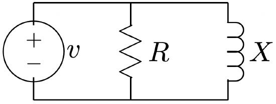Figure 14: Example Circuit

of 120 volts and \(\ R\) and \(\ X\) are both 100 Ω. Then:

\(\ v(t)=170 \cos \omega t\)

The admittance of this network is:

\(\ Y=\frac{1}{100}-\frac{j}{100}\)

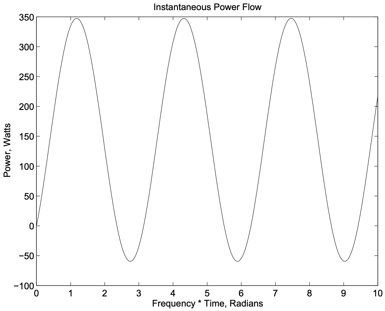Figure 15: Power Flow For Example Circuit

so that the complex amplitude of current is:

\(\ I=1.7-j 1.7\)

And then complex power is:

\(\ P+j Q=\frac{1}{2} 170(1.7+j 1.7)\)

Real and reactive power are, respectively: \(\ P=144 \mathrm{~W}\), \(\ Q=144 \mathrm{VAR}\). This gives a power factor angle of \(\ \psi=\arctan (1)=45^{\circ}\). Then, instantaneous power is:

\(\ p=144\left[1+\cos 2\left(\omega t-45^{\circ}\right)\right]+144 \sin 2\left(\omega t-45^{\circ}\right)\)

This is illustrated in Figure 15.