2.9: Power Flow Through An Impedance

Consider the situation shown in Figure 16. This actually represents a number of important situations in power systems, where the impedance \(\ \underline{Z}\) might represent a transmission line, transformer or motor winding. Of interest to us is the flow of power through the impedance. Current is given

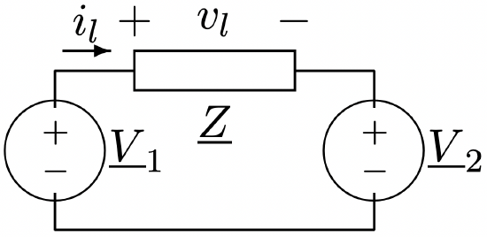Figure 16: Power Flow Example

by:

\[\ \underline{i_{l}}=\frac{\underline{V}_{1}-\underline{V}_{2}}{\underline{Z}}\label{72} \]

Then, complex power flow out of the left- hand voltage source is:

\[\ P+j Q=\frac{1}{2} \underline{V}_{1}\left(\frac{\underline{V}_{1}^{*}-\underline{V}_{2}^{*}}{\underline{Z}^{*}}\right)\label{73} \]

Now, the complex amplitudes may be expressed as:

\[\ \underline{V}_{1}=\left|\underline{V}_{1}\right| e^{j \theta}\label{74} \]

\[\ \underline{V}_{2}=\left|\underline{V}_{2}\right| e^{j \theta+\delta}\label{75} \]

where \(\ \delta\) is the relative phase angle between the two voltage sources. Complex power at the terminals of the voltage source \(\ \underline{V}_{1}\) is now given by:

\[\ P+j Q=\frac{\left|\underline{V}_{1}\right|^{2}}{2 \underline{Z}^{*}}-\frac{\left|\underline{V}_{1}\right|\left|\underline{V}_{2}\right| e^{-j \delta}}{2 \underline{Z}^{*}}\label{76} \]

This is describable as a circle in the complex plane, with its origin at

\(\ \frac{\left|\underline{V}_{1}\right|^{2}}{2 \underline{Z}^{*}}\)

and its radius equal to:

\(\ \frac{\left|\underline{V}_{1}\right|\left|\underline{V}_{2}\right|}{2|\underline{Z}|}\)

Now suppose the impedance through which we are passing power is describable as a simple inductance as shown in Figure 17. This is perhaps the simplest of transmission line models which represents only the inductive impedance of the line. Line inductance arises because currents in the line produce magnetic fields, and this is a fair model for most lines which are fairly ’short’. More on that in the next section. This line has the impedance

\(\ Z=j \omega L=j X_{L}\)

Now, switching to RMS amplitudes, so that \(\ \underline{V}_{s}=\sqrt{2} \underline{V}_{1}\) and \(\ \underline{V}_{r}=\sqrt{2} \underline{V}_{2}\), Then real and reactive power flow are:

\(\ \begin{aligned}
P_{s}+j Q_{s} &=\underline{V}_{s} \underline{I}^{*}=j \frac{\left|V_{s}\right|^{2}-\underline{V}_{s} \underline{V}_{r}^{*}}{X_{l}} \\
P_{r}+j Q_{r} &=-\underline{V}_{r} \underline{I}^{*}=j \frac{\left|V_{r}\right|^{2}-\underline{V}_{s}^{*} \underline{V}_{r}}{X_{l}}
\end{aligned}\)

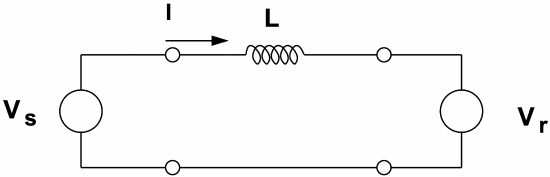Figure 17: Simplest Transmission Line Model

Now if we assume that the voltages are of the form:

\(\ \begin{array}{l}
\underline{V}_{s}=V_{s} e^{j \phi} \\
\underline{V}_{r}=V_{r} e^{j \theta}
\end{array}\)

and that the relative phase angle between them is \(\ \phi-\theta=\delta\) and doing a little trig:

\(\ \begin{aligned}
P_{s} &=\frac{V_{s} V_{r} \sin \delta}{X_{L}} \\
Q_{s} &=\frac{V_{s}^{2}-V_{s} V_{r} \cos \delta}{X_{L}} \\
P_{r} &=-\frac{V_{s} V_{r} \sin \delta}{X_{L}} \\
Q_{r} &=\frac{V_{r}^{2}-V_{s} V_{r} \cos \delta}{X_{L}}
\end{aligned}\)

A picture of this locus is referred to as a power circle diagram, because of its shape. Figure 18 shows the construction of a sending end power circle diagram for equal sending-end and receivingend voltages and a purely reactive impedance.

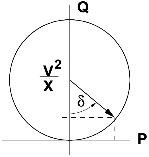Figure 18: Power Circle, Equal Voltages

As a check, consider the reactive power consumed by the line itself: we expect that \(\ Q_{s}+Q_{r}=Q_L\), and so:

\(\ Q_{s}+Q_{r}=\frac{V_{s}^{2}+V_{r}^{2}-2 V_{s} V_{r} \cos \delta}{X_{L}}\)

Note that the voltage across the line element itself is found using the law of cosines (see Figure 19:

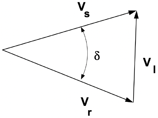Figure 19: Illustration of the Law of Cosines

\(\ V_{L}^{2}=V_{s}^{2}+V_{r}^{2}-2 V_{s} V_{r} \cos \delta\)

and, indeed,

\(\ Q_{L}=\frac{V_{L}^{2}}{X_{L}}\)