
6.2: Magnetic Circuits
- Page ID
- 55588

As it turns out, magnetic circuits are very similar and are governed by laws that are not at all different from those of electric circuits, with only one minor difference.
Conservation of Flux: Gauss’ Law
To start, Gauss’ law is:
\(\ \oiint \vec{B} \cdot d \vec{a}=0\)
This reflects that notion that there are no sources of flux: this is a truely sinusoidal quantity. It neither begins nor ends but just goes in circles.
If we note a fraction of the surface around a node and call it surface k, the flux through that surface is:
\(\ \Phi_{k}=\iint \ _{A_{k}} \vec{B} \cdot d \vec{a}\)
If we take the sum of all partial fluxes through a surface surrounding a note we come to the analog of KCL:
\(\ \sum_{k} \Phi_{k}=0\)
MMF: Ampere’s Law
Ampere’s Law is simply stated as:
\(\ \oint \vec{H} \cdot d \ell=\iint \vec{J} \cdot d \vec{a}\)
The integral of current density \(\ \vec{J}\) is current, quantified in the SI system as Amperes. As it is generally carried in wires which might number, say , \(\ N\), it is often quantified as:
\(\ \iint \vec{J} \cdot d \vec{a}=N I\)
For this we will often use the term MagnetoMotive Force or MMF, which gets the symbol \(\ F\). If we use that symbol to denote the integral of magnetic field over a magnetic circuit element:
\(\ F_{k}=\int_{a_{k}}^{b_{k}} \vec{H} \cdot d \vec{\ell}\)
Then, if we take enough of these subintegrals to cover the loop around a group of elements, we have
\(\ \sum_{k} F_{k}=N I\)
Note that this is not exactly the same as KVL, as it has a source term on the right.
Magnetic Circuit Element: Analogy to Ohm’s Law
Magnetic circuits have an equivalent to resistance. It is the ratio of MMF to flux and has the symbol \(\ \mathcal{R}\). I direct comparison with the derivation of resistance, a magnetic circuit element is shown in Figure 2.
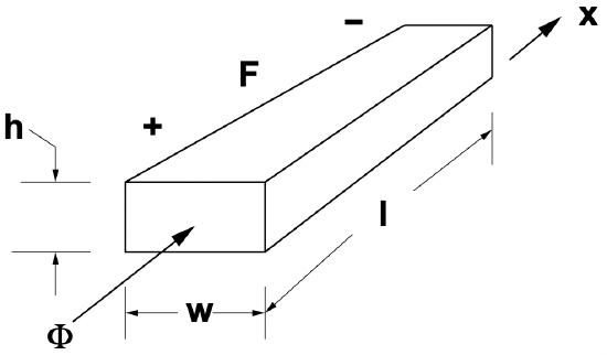 Figure 2: Magnetic circuit element
Assume that the material of this element has permeability \(\ \mu>\mu_{0}\), so that it has a constitutive relationship:
\(\ B_{x}=\mu H_{x}\)
If flux density in the material is uniform, total flux through the element is:
\(\ \Phi=h w B_{x}=h w \mu H_{x}\)
And the MMF is simply the integral of magnetic field H from one end to the other: again we assume uniformity so that:
\(\ F=\ell H_{x}\)
The reluctance of this element is then:
\(\ \mathcal{R}=\frac{F}{\Phi}=\frac{\ell}{h w \mu}\)
Magnetic Gaps
In reality, magnetic circuits tend to be made up of very highly permeable elements (pieces of iron) and relatively small air-gaps. A sketch of such a gap is shown in Figure 3.
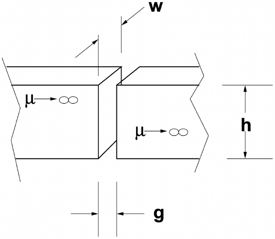 Figure 3: Gap between magnetic elements
It is usually permissible to assume that iron elements have very high permeability \(\ (\mu \rightarrow \infty)\), so that there is negligible MMF drop. In this sense the iron elements serve in the same role as copper or aluminum wire in electric circuits. The gap, on the other hand, has reluctance:
\(\ \mathcal{R}_{g}=\frac{g}{h w \mu_{0}}\)
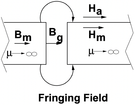 Figure 4: Gap details
Boundary Conditions
Shown in Figure 4 is the cross-section of a gap. It is assumed that the elements shown have some depth into the paper which is greater than the gap width \(\ g\). If the permeability of the elements to the right and the left is very high, we say that magnetic flux is largely confined to those elements. Note that the boundary condition associated with Ampere’s Law dictates that the magnetic field intensity \(\ H_{a}\) in the air adjacent to the permeable material and parallel with the surface must be equal to the magnetic field intensity \(\ H_{m}\) just inside the magnetic material and parallel with the surface. If the material is very highly permeable \(\ (\mu \rightarrow \infty)\), that magnetic field must be nearly zero: \(\ H_{a}=H_{m} \rightarrow 0\). This means that magnetic field must be perpendicular to the surface of very highly permeable material. This is the case in the gap itself, where:
\(\ B_{g}=B_{m}\)
We should note, however, that there will be ’fringing’ fields in the region near the gap, so that our expression for the reluctance of the gap will not be quite correct. The accuracy of the expression which ignores fringing is best for really small gaps and generally over-estimates the reluctance.