
5: Active Mode Locking
- Page ID
- 44655
\( \newcommand{\vecs}[1]{\overset { \scriptstyle \rightharpoonup} {\mathbf{#1}} } \)
\( \newcommand{\vecd}[1]{\overset{-\!-\!\rightharpoonup}{\vphantom{a}\smash {#1}}} \)
\( \newcommand{\dsum}{\displaystyle\sum\limits} \)
\( \newcommand{\dint}{\displaystyle\int\limits} \)
\( \newcommand{\dlim}{\displaystyle\lim\limits} \)
\( \newcommand{\id}{\mathrm{id}}\) \( \newcommand{\Span}{\mathrm{span}}\)
( \newcommand{\kernel}{\mathrm{null}\,}\) \( \newcommand{\range}{\mathrm{range}\,}\)
\( \newcommand{\RealPart}{\mathrm{Re}}\) \( \newcommand{\ImaginaryPart}{\mathrm{Im}}\)
\( \newcommand{\Argument}{\mathrm{Arg}}\) \( \newcommand{\norm}[1]{\| #1 \|}\)
\( \newcommand{\inner}[2]{\langle #1, #2 \rangle}\)
\( \newcommand{\Span}{\mathrm{span}}\)
\( \newcommand{\id}{\mathrm{id}}\)
\( \newcommand{\Span}{\mathrm{span}}\)
\( \newcommand{\kernel}{\mathrm{null}\,}\)
\( \newcommand{\range}{\mathrm{range}\,}\)
\( \newcommand{\RealPart}{\mathrm{Re}}\)
\( \newcommand{\ImaginaryPart}{\mathrm{Im}}\)
\( \newcommand{\Argument}{\mathrm{Arg}}\)
\( \newcommand{\norm}[1]{\| #1 \|}\)
\( \newcommand{\inner}[2]{\langle #1, #2 \rangle}\)
\( \newcommand{\Span}{\mathrm{span}}\) \( \newcommand{\AA}{\unicode[.8,0]{x212B}}\)
\( \newcommand{\vectorA}[1]{\vec{#1}} % arrow\)
\( \newcommand{\vectorAt}[1]{\vec{\text{#1}}} % arrow\)
\( \newcommand{\vectorB}[1]{\overset { \scriptstyle \rightharpoonup} {\mathbf{#1}} } \)
\( \newcommand{\vectorC}[1]{\textbf{#1}} \)
\( \newcommand{\vectorD}[1]{\overrightarrow{#1}} \)
\( \newcommand{\vectorDt}[1]{\overrightarrow{\text{#1}}} \)
\( \newcommand{\vectE}[1]{\overset{-\!-\!\rightharpoonup}{\vphantom{a}\smash{\mathbf {#1}}}} \)
\( \newcommand{\vecs}[1]{\overset { \scriptstyle \rightharpoonup} {\mathbf{#1}} } \)
\(\newcommand{\longvect}{\overrightarrow}\)
\( \newcommand{\vecd}[1]{\overset{-\!-\!\rightharpoonup}{\vphantom{a}\smash {#1}}} \)
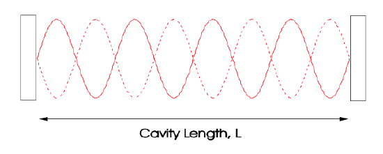
\(\newcommand{\avec}{\mathbf a}\) \(\newcommand{\bvec}{\mathbf b}\) \(\newcommand{\cvec}{\mathbf c}\) \(\newcommand{\dvec}{\mathbf d}\) \(\newcommand{\dtil}{\widetilde{\mathbf d}}\) \(\newcommand{\evec}{\mathbf e}\) \(\newcommand{\fvec}{\mathbf f}\) \(\newcommand{\nvec}{\mathbf n}\) \(\newcommand{\pvec}{\mathbf p}\) \(\newcommand{\qvec}{\mathbf q}\) \(\newcommand{\svec}{\mathbf s}\) \(\newcommand{\tvec}{\mathbf t}\) \(\newcommand{\uvec}{\mathbf u}\) \(\newcommand{\vvec}{\mathbf v}\) \(\newcommand{\wvec}{\mathbf w}\) \(\newcommand{\xvec}{\mathbf x}\) \(\newcommand{\yvec}{\mathbf y}\) \(\newcommand{\zvec}{\mathbf z}\) \(\newcommand{\rvec}{\mathbf r}\) \(\newcommand{\mvec}{\mathbf m}\) \(\newcommand{\zerovec}{\mathbf 0}\) \(\newcommand{\onevec}{\mathbf 1}\) \(\newcommand{\real}{\mathbb R}\) \(\newcommand{\twovec}[2]{\left[\begin{array}{r}#1 \\ #2 \end{array}\right]}\) \(\newcommand{\ctwovec}[2]{\left[\begin{array}{c}#1 \\ #2 \end{array}\right]}\) \(\newcommand{\threevec}[3]{\left[\begin{array}{r}#1 \\ #2 \\ #3 \end{array}\right]}\) \(\newcommand{\cthreevec}[3]{\left[\begin{array}{c}#1 \\ #2 \\ #3 \end{array}\right]}\) \(\newcommand{\fourvec}[4]{\left[\begin{array}{r}#1 \\ #2 \\ #3 \\ #4 \end{array}\right]}\) \(\newcommand{\cfourvec}[4]{\left[\begin{array}{c}#1 \\ #2 \\ #3 \\ #4 \end{array}\right]}\) \(\newcommand{\fivevec}[5]{\left[\begin{array}{r}#1 \\ #2 \\ #3 \\ #4 \\ #5 \\ \end{array}\right]}\) \(\newcommand{\cfivevec}[5]{\left[\begin{array}{c}#1 \\ #2 \\ #3 \\ #4 \\ #5 \\ \end{array}\right]}\) \(\newcommand{\mattwo}[4]{\left[\begin{array}{rr}#1 \amp #2 \\ #3 \amp #4 \\ \end{array}\right]}\) \(\newcommand{\laspan}[1]{\text{Span}\{#1\}}\) \(\newcommand{\bcal}{\cal B}\) \(\newcommand{\ccal}{\cal C}\) \(\newcommand{\scal}{\cal S}\) \(\newcommand{\wcal}{\cal W}\) \(\newcommand{\ecal}{\cal E}\) \(\newcommand{\coords}[2]{\left\{#1\right\}_{#2}}\) \(\newcommand{\gray}[1]{\color{gray}{#1}}\) \(\newcommand{\lgray}[1]{\color{lightgray}{#1}}\) \(\newcommand{\rank}{\operatorname{rank}}\) \(\newcommand{\row}{\text{Row}}\) \(\newcommand{\col}{\text{Col}}\) \(\renewcommand{\row}{\text{Row}}\) \(\newcommand{\nul}{\text{Nul}}\) \(\newcommand{\var}{\text{Var}}\) \(\newcommand{\corr}{\text{corr}}\) \(\newcommand{\len}[1]{\left|#1\right|}\) \(\newcommand{\bbar}{\overline{\bvec}}\) \(\newcommand{\bhat}{\widehat{\bvec}}\) \(\newcommand{\bperp}{\bvec^\perp}\) \(\newcommand{\xhat}{\widehat{\xvec}}\) \(\newcommand{\vhat}{\widehat{\vvec}}\) \(\newcommand{\uhat}{\widehat{\uvec}}\) \(\newcommand{\what}{\widehat{\wvec}}\) \(\newcommand{\Sighat}{\widehat{\Sigma}}\) \(\newcommand{\lt}{<}\) \(\newcommand{\gt}{>}\) \(\newcommand{\amp}{&}\) \(\definecolor{fillinmathshade}{gray}{0.9}\)For simplicity, we assume, that the laser operates in the transverse fundamental modes and, therefore, we only have to treat the longitudinal modes of the laser similar to a simple plane parallel Fabry-Perot resonator (Figure: 5.1). We consider one polarization of the field only, however, as we will say later for some mode-locked laser polarization dynamics will become important.
The task of mode-locking is to get as many of the longitudinal modes lasing in a phase synchronous fashion, such that the superposition of all modes represents a pulse with a spatial extent much shorter than the cavity. The pulse will then propagate at the group velocity corresponding to the center frequency of the pulse.
- 5.1: The Master Equation of Mode Locking
- This page explores intracavity field behavior in cold cavities, highlighting wave superpositions influenced by boundary conditions and introducing a gradually varying field envelope tied to pulse propagation equations, including gain and loss effects. It also discusses the master equation for modelocking in optical modulators, focusing on linear and nonlinear effects on light pulses, emphasizing the significance of these influences on pulse shape and dynamics in optical systems.
- 5.2: Active Mode Locking by Loss Modulation
- This page explores active mode locking in lasers, initiated by Kuizenga and Siegman in 1970, using Haus's master equation to describe laser pulse behavior. It details how periodic modulation of intracavity loss synchronizes with round-trip time, resulting in Gaussian pulses with widths between 10-100 ps and a time-bandwidth product of 0.44.
- 5.3: Active Mode-Locking by Phase Modulation
- This page explores sideband generation via phase modulation, emphasizing its out-of-phase relationship with the carrier and the associated chirp effect in steady-state pulses. It details modifications to the master equation for modelocking analysis and discusses the influence of complex parameter \(\tau_a'\) on pulse characteristics.
- 5.4: Active Mode Locking with Additional SPM
- This page explores the effects of self-phase modulation (SPM) in actively mode-locked lasers, presenting the governing master equation and noting the lack of analytic solutions. It discusses SPM's influence on pulse chirp and provides equations for determining pulse width and excess gain. Although SPM initially reduces pulse width, it can induce instability, prompting the need for stabilization techniques like negative group delay dispersion to achieve soliton formation.
- 5.5: 5.5 Active Mode Locking with Soliton Formation
- This page provides an in-depth analysis of soliton behavior in fiber and solid-state lasers, focusing on the effects of negative group delay dispersion (GDD) and self-phase modulation on pulse width reduction and stability. It discusses critical conditions for soliton existence and the interplay between gain dynamics and continuum fields.
- 5.6: Summary
- This page explores the outcomes of pure active mode-locking in lasers, producing Gaussian pulses with widths related to gain bandwidth. It explains how phase modulators create chirped Gaussian pulses while solitons can be stabilized through active mode locking. The implications for passive mode locking are discussed, indicating that a slow saturable absorber with a longer recovery time than the soliton pulse width can effectively achieve mode locking.
- 5.7: Active Modelocking with Detuning
- This page examines the complexities of achieving synchronism in actively modelocked lasers, emphasizing the impact of detuning on stability and system dynamics. It discusses the relationship between detuning and hydrodynamic transitions, the role of eigenmodes, and the sensitivity of nonnormal systems. The text highlights simulations demonstrating how pulse dynamics transition to chaos at higher detuning levels and explores the critical detuning threshold influenced by gain saturation.