7.3: Scattering Parameters

Direct measurement of the \(z\) and \(y\) parameters requires that the ports be terminated in either short or open circuits. For active circuits this could result in undesired behavior, including oscillation or destruction. Also, at RF it is difficult to realize a good open or short. Since RF circuits are designed with close attention to maximum power transfer conditions, resistive terminations are preferred, as these are closer to the actual operating conditions. Thus the effect of measurement errors will have less impact. This is the way scattering parameters are measured.

The discussion of scattering parameters, \(S\) parameters\(^{1}\), begins by considering the reflection coefficient, which is the \(S\) parameter of a one-port network.

7.3.1 Reflection Coefficient

The reflection coefficient, \(\Gamma\), of a load \(\Gamma_{L}\) can be determined by separately measuring the forward- and backward-traveling voltages on a transmission line terminated by the load:

\[\label{eq:1}\Gamma (x)=\frac{V^{-}(x)}{V^{+}(x)} \]

Imagine between the source and the load that there is a line of characteristic impedance \(Z_{0}\) and with infinitesimal length, then \(\Gamma\) at the load is related to the impedance \(Z_{L}\) by

\[\label{eq:2}\Gamma (0)=\frac{Z_{L}-Z_{0}}{Z_{L}+Z_{0}} \]

where \(Z_{0}\) is the characteristic impedance of the connecting transmission line. This can also be written as

\[\label{eq:3}\Gamma (0)=\frac{Y_{0}-Y_{L}}{Y_{0}+Y_{L}} \]

where \(Y_{0} = 1/Z_{0}\) and \(Y_{L} = 1/Z_{L}\). More completely, \(\Gamma\) as defined above is called the voltage reflection coefficient sometimes denoted \(\Gamma^{V}\).

Recall that the current reflection coefficient \(\Gamma^{I} = −\Gamma^{V}\).

7.3.2 Two Port \(S\) Parameters

Two-port \(S\) parameters are defined in terms of traveling waves on transmission lines with real characteristic impedance \(Z_{0}\) attached to each of the ports of a network, see Figure 7.2.1(b):

\[\label{eq:4}V_{1}^{-}=S_{11}V_{1}^{+}+S_{12}V_{2}^{+} \]

\[\label{eq:5}V_{2}^{-}=S_{21}V_{1}^{+}+S_{22}V_{2}^{+} \]

where \(S_{ij}\) are the individual \(S\) parameters. In matrix form

\[\label{eq:6}\left[\begin{array}{l}{V_{1}^{-}}\\{V_{2}^{-}}\end{array}\right]=\left[\begin{array}{ll}{S_{11}}&{S_{12}}\\{S_{21}}&{S_{22}}\end{array}\right] \left[\begin{array}{l}{V_{1}^{+}}\\{V_{2}^{+}}\end{array}\right] =\mathbf{S}\left[\begin{array}{l}{V_{1}^{+}}\\{V_{2}^{+}}\end{array}\right] \]

Individual \(S\) parameters are determined by measuring the forward- and backward-traveling waves with loads \(Z_{0}\) at the ports. Since the load is \(Z_{0}\) it cannot reflect power and so \(V_{2}^{+}= 0\), then

\[\label{eq:7}S_{11}=\left. \frac{V_{1}^{-}}{V_{1}^{+}}\right| _{V_{2}^{+}=0} \]

The remaining parameters are determined similarly and so S22 is found as

\[\label{eq:8}S_{22}=\left. \frac{V_{2}^{-}}{V_{2}^{+}}\right| _{V_{1}^{+}=0} \]

and the transmission parameter as

\[\label{eq:9}S_{21}=\left. \frac{V_{2}^{-}}{V_{1}^{+}}\right| _{V_{2}^{+}=0} \]

	\(S\)	In terms of \(S\)
\(z\)	\(Z_{11}'=z_{11}Z_{0}\quad Z_{12}'=z_{12}Z_{0}\)	\(Z_{21}'=z_{21}Z_{0}\quad Z_{22}'=z_{22}Z_{0}\)
	\(\begin{aligned} \delta_{z}&= (1+z_{11})(1+z_{22})-z_{12}z_{21} \\ S_{11}&=[(z_{11}-1)(z_{22}+1)-z_{12}z_{21}]/\delta_{z} \\ S_{12}&=2z_{12}/\delta_{z} \\ S_{21}&=2z_{21}/\delta_{z} \\ S_{22}&=[(z_{11}+1)(z_{22}-1)-z_{12}z_{21}]/\delta_{z}\end{aligned}\)	\(\begin{aligned}\delta_{S}&=(1-S_{11})(1-S_{22})-S_{12}S_{21} \\ z_{11}&=[(1+S_{11})(1-S_{22})+S_{12}S_{21}]/\delta_{S} \\ z_{12}&=2S_{12}/\delta_{S} \\ z_{21}&=2S_{21}/\delta_{S} \\ z_{22}&=[(1-S_{11})(1+S_{22})+S_{12}S_{21}]/\delta_{S}\end{aligned}\)
\(y\)	\(Y_{11}'=y_{11}/Z_{0}\quad Y_{12}'=y_{12}/Z_{0}\)	\(Y_{21}'=y_{21}/Z_{0}\quad Y_{22}'=y_{22}/Z_{0}\)
	\(\begin{aligned}\delta_{y}&=(1+y_{11})(1+y_{22})-y_{12}y_{21} \\ S_{11}&=[(1-y_{11})(1+y_{22})+y_{12}y_{21}]/\delta_{y} \\ S_{12}&=-2y_{12}/\delta_{y} \\ S_{21}&=-2y_{21}/\delta_{y} \\ S_{22} &=[(1+y_{11})(1-y_{22})+y_{12}y_{21}]/\delta_{y}\end{aligned}\)	\(\begin{aligned}\delta_{S}&=(1+S_{11})(1+S_{22})-S_{12}S_{21}\\ y_{11}&=[(1-S_{11})(1+S_{22})+S_{12}S_{21}]/\delta_{S} \\ y_{12}&=-2S_{12}/\delta_{S} \\ y_{21}&=-2S_{21}/\delta_{S} \\ y_{22}&=[(1+S_{11})(1-S_{22})+S_{12}S_{21}]/\delta_{S}\end{aligned}\)

Table \(\PageIndex{1}\): Two-port \(S\) parameter conversion chart. The \(z\), and \(y\) parameters are normalized to \(Z_{0}\). \(Z′\) and \(Y′\) are the actual parameters.

In the reverse direction,

\[\label{eq:10}S_{12}=\left. \frac{V_{1}^{-}}{V_{2}^{+}}\right| _{V_{1}^{+}=0} \]

In the above \(Z_{0}\) is referred to as the normalization impedance or equivalently the reference impedance. In some circumstances \(Z_{\text{REF}}\) is used to denote reference impedance to avoid possible confusion with a transmission line impedance that is not the same as the reference impedance. The \(S\) parameters here are also called normalized \(S\) parameters, and the \(S\) parameters are normalized to the same real reference impedance at each port.

The relationships between the two-port \(S\) parameters and the common network parameters are given in Table \(\PageIndex{1}\). It is interesting to note that \(S_{21}/S_{12} = z_{21}/z_{12} = y_{21}/y_{12}\). That is, the ratio of the forward to reverse parameters (at least for \(S,\: z,\) and \(y\) parameters) are the same and this ratio is one for a reciprocal device. An \(S\) parameter is a voltage ratio, so when it is expressed in decibels \(S_{ij}|_{\text{ dB}} = 20\log (S_{ij})\).

A reciprocal network has \(S_{12} = S_{21}\). If unit power flows into a two-port, a fraction, \(|S_{11}|^{2}\), is reflected and a further fraction, \(|S_{21}|^{2}\), is transmitted through the network.

Example \(\PageIndex{1}\): Two-Port \(S\) Parameters

What are the \(S\) parameters of a \(30\text{ dB}\) attenuator?

Solution

An attenuator is shown with a system impedance of \(Z_{0}\). An ideal attenuator has no reflection at each of the two ports when the attenuator is embedded in its system impedance. Thus \(\Gamma_{\text{in}} =0=\Gamma_{\text{out}}\). Since there is no reflection from the load or the source, this implies that \(S_{11}=0=S_{22}\).

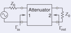
Figure \(\PageIndex{1}\)

Since this is a \(30\text{ dB}\) attenuator, the power delivered to the load impedance \(Z_{0}\) is \(30\text{ dB}\) below the power available from the source, thus \(S_{21} = −30\text{ dB} = 0.0316\). The attenuator is reciprocal and so \(S_{12} = S_{21}\). Thus the \(S\) parameters of the attenuator are

\[\label{eq:11}\mathbf{S}=\left[\begin{array}{cc}{0}&{0.0316}\\{0.0316}&{0}\end{array}\right] \]

Note that the reference impedance did not need to be known to develop the \(S\) parameters.

7.3.3 Input Reflection Coefficient of a Terminated Two-Port Network

A two-port is shown in Figure \(\PageIndex{1}\) that is terminated at Port 2 in a load with a reflection coefficient \(\Gamma_{L}\). The lines at each of the ports are of infinitesimal length (i.e., \(\ell_{1}\to 0\) and \(\ell_{2}\to 0\)) and are used to make it easier to visualize the separation of the voltage into forward- and backward-traveling components. The aim in this section is to develop a formula for the input reflection coefficient \(\Gamma_{\text{in}} = V_{1}^{-}/V_{1}^{+}\). For the circuit in Figure \(\PageIndex{1}\), three equations can be developed:

\[\label{eq:12}V_{1}^{-}=S_{11}V_{1}^{+}+S_{12}V_{2}^{+} \]

\[\label{eq:13}V_{2}^{-}=S_{21}V_{1}^{+}+S_{22}V_{2}^{+} \]

\[\label{eq:14}V_{2}^{+}=\Gamma_{L}V_{2}^{-},\quad\text{i.e.,}\quad V_{2}^{-}=V_{2}^{+}/\Gamma_{L} \]

Note that \(V_{2}^{-}\) is the voltage wave that leaves the two-port but is incident on the load \(\Gamma_{L}\). The aim here is to eliminate \(V_{2}^{+}\) and \(V_{2}^{-}\). Substituting Equation \(\eqref{eq:14}\) into Equation \(\eqref{eq:13}\) leads to

\[\label{eq:15}V_{2}^{+}/\Gamma_{L}=S_{21}V_{1}^{+}+S_{22}V_{2}^{+} \]

\[\label{eq:16}V_{2}^{+}\left(\frac{1-S_{22}\Gamma_{L}}{\Gamma_{L}}\right)=S_{21}V_{1}^{+} \]

\[\label{eq:17}V_{2}^{+}=\left(\frac{S_{21}\Gamma_{L}}{1-S_{22}\Gamma_{L}}\right)V_{1}^{+} \]

Now substituting Equation \(\eqref{eq:17}\) in Equation \(\eqref{eq:12}\) yields

\[\label{eq:18}V_{1}^{-}=S_{11}V_{1}^{+}+S_{12}\left(\frac{S_{21}\Gamma_{L}}{1-S_{22}\Gamma_{L}}\right)V_{1}^{+} \]

and so

\[\label{eq:19}\Gamma_{\text{in}}=S_{11}+\frac{S_{12}S_{21}\Gamma_{L}}{1-S_{22}\Gamma_{L}} \]

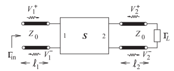
Figure \(\PageIndex{1}\): A terminated two-port network with transmission lines of infinitesimal length at the ports.

7.3.4 Properties of a Two-Part in Terms of \(S\) Parameters

The properties of most interest are whether the two-port network is lossless, passive, or reciprocal.

If a network is lossless, all of the power input to the network must leave the network. The power incident on Port 1 of a network is

\[\label{eq:20}P_{1}^{+}=\left|\frac{\frac{1}{2}V_{1}^{+}}{Z_{0}}\right|^{2} \]

and the power leaving Port 1 is

\[\label{eq:21}P_{1}^{-}=\left|\frac{\frac{1}{2}V_{1}^{-}}{Z_{0}}\right|^{2} \]

This can be repeated for Port 2 and the factor \(\frac{1}{2}/Z_{0}\) appears in all expressions. So cancelling this factor, the condition for the network to be lossless is

\[\label{eq:22}|S_{11}|^{2}+|S_{21}|^{2}=1\quad\text{and}\quad |S_{12}|^{2}+|S_{22}|^{2}=1 \]

For a network to be passive, no more power can leave the network than enters it. So the condition for passivity is

\[\label{eq:23}|S_{11}|^{2}+|S_{21}|^{2}\leq 1\quad\text{and}\quad |S_{12}|^{2}+|S_{22}|^{2}\leq 1 \]

Reciprocity requires that \(S_{21} = S_{12}\).

Footnotes

[1] For historical reasons a capital “S” is used when referring to \(S\) parameters. For most other network parameters, lowercase is used (e.g., \(z\) parameters for impedance parameters).