
5.2: Telegrapher's Equations
- Page ID
- 88557

Let's look at just one little section of the line, and define some voltages and currents as in Figure \(\PageIndex{1}\).
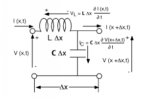 Figure \(\PageIndex{1}\): Applying Kirchoff's Laws

For the section of line \(Delta x\) long, the voltage at its input is just \(V(x, t)\) and the voltage at the output is \(V(x + \Delta x, t)\). Likewise, we have a current \(I(x, t)\) entering the section, and another current \(I(x + \Delta x, t)\) leaving the section of line. Note that both the voltage and the current are functions of time as well as position.
The voltage drop across the inductor is just: \[V_{L} = \mathbf{L} \Delta (x) \frac{\partial I(x, t)}{\partial t}\]
Likewise, the current flowing down through the capacitor is \[I_{C} = \mathbf{C} \Delta (x) \frac{\partial V(x + \Delta (x), t)}{\partial t}\]
Now we do a KVL around the outside of the section of line and we get \[V(x, t) - V_{L} - V(x + \Delta (x), t) = 0\]
Substituting Equation \(\PageIndex{1}\) for \(V_{L}\) and taking it over to the right hand side, we have \[V(x, t) - V(x + \Delta (x), t) = \mathbf{L} \Delta (x) \frac{\partial I(x, t)}{\partial t}\]
Let's multiply this by \(-1\), and bring the \(\Delta (x)\) over to the left hand side. \[\frac{V(x + \Delta (x), t) - V(x, t)}{\Delta (x)} = - \left( \mathbf{L} \frac{\partial I(x, t)}{\partial t}\right)\]
We take the limit as \(\Delta (x) \rightarrow 0\) and the LHS becomes a derivative: \[\frac{\partial V(x, t)}{\partial x} = - \left(\mathbf{L} \frac{\partial I(x, t)}{\partial t}\right)\]
Now we can do a KCL at the node where the inductor and capacitor come together. \[I(x, t) - \mathbf{C} \Delta (x) \frac{\partial V(x + \Delta (x), t)}{\partial t} - I(x + \Delta (x), t) = 0\]
And upon rearrangement: \[\frac{I(x + \Delta (x), t) - I(x, t)}{\Delta (x)} = -\left(\mathbf{C} \frac{\partial V(x + \Delta (x), t)}{\partial t}\right)\]
Now when we let \(\Delta (x) \rightarrow 0\), the left hand side again becomes a derivative, and on the right hand side \(V(x + \Delta (x), t) \rightarrow V(x, t)\), so we have: \[\frac{\partial V(x, t)}{\partial x} = - \left(\mathbf{C} \frac{\partial V(x, t)}{\partial t}\right)\]
Equation \(\PageIndex{6}\) and Equation \(\PageIndex{9}\) are so important we will write them out again together: \[\frac{\partial V(x, t)}{\partial x} = -\left(\mathbf{L} \frac{\partial I(x, t)}{\partial t}\right)\] \[\frac{\partial I(x, t)}{\partial x} = -\left(\mathbf{C} \frac{\partial V(x, t)}{\partial t}\right)\]
These are called the telegrapher's equations, and they are all we really need to derive how electrical signals behave as they move along on transmission lines. Note what they say. The first one says that at some point \(x\) along the line, the incremental voltage drop that we experience as we move down the line is just the distributed inductance \(\mathbf{L}\) times the time derivative of the current flowing in the line at that point. The second equation simply tells us that the loss of current as we go down the line is proportional to the distributed capacitance \(\mathbf{C}\) times the time rate of change of the voltage on the line. As you should be easily aware, what we have here are a pair of coupled linear differential equations in time and position for \(V(x, t)\) and \(I(x, t)\).