5.5: Exciting a Line

Last updated
Save as PDF

Page ID: 88560

\( \newcommand{\vecs}[1]{\overset { \scriptstyle \rightharpoonup} {\mathbf{#1}} } \) \( \newcommand{\vecd}[1]{\overset{-\!-\!\rightharpoonup}{\vphantom{a}\smash {#1}}} \)\(\newcommand{\id}{\mathrm{id}}\) \( \newcommand{\Span}{\mathrm{span}}\) \( \newcommand{\kernel}{\mathrm{null}\,}\) \( \newcommand{\range}{\mathrm{range}\,}\) \( \newcommand{\RealPart}{\mathrm{Re}}\) \( \newcommand{\ImaginaryPart}{\mathrm{Im}}\) \( \newcommand{\Argument}{\mathrm{Arg}}\) \( \newcommand{\norm}[1]{\| #1 \|}\) \( \newcommand{\inner}[2]{\langle #1, #2 \rangle}\) \( \newcommand{\Span}{\mathrm{span}}\) \(\newcommand{\id}{\mathrm{id}}\) \( \newcommand{\Span}{\mathrm{span}}\) \( \newcommand{\kernel}{\mathrm{null}\,}\) \( \newcommand{\range}{\mathrm{range}\,}\) \( \newcommand{\RealPart}{\mathrm{Re}}\) \( \newcommand{\ImaginaryPart}{\mathrm{Im}}\) \( \newcommand{\Argument}{\mathrm{Arg}}\) \( \newcommand{\norm}[1]{\| #1 \|}\) \( \newcommand{\inner}[2]{\langle #1, #2 \rangle}\) \( \newcommand{\Span}{\mathrm{span}}\)\(\newcommand{\AA}{\unicode[.8,0]{x212B}}\)

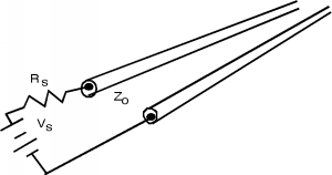
We will now go on and look at what happens when we excite the line. Let's take a DC voltage source with a source internal impedance \(R_{s}\) and connect it to our semi-infinite line. The sketch in Figure \(\PageIndex{1}\) is sort of awkward-looking and will be hard to analyze, so let's make a more "schematic like" drawing in Figure \(\PageIndex{1}\), keeping in mind that it is a situation such as the one in Figure \(\PageIndex{1}\) which we trying to represent.

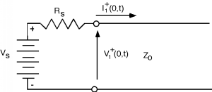
A transmission line consists of two wires, each with an impedance of Z_0, stretching into the page. The wire on the right connects to the negative end of a voltage source v_s, and the positive end of the source connects to a resistor R_s and then the wire on the left in series. — Figure \(\PageIndex{1}\): Exciting a transmission line

Two horizontal lines are connected at their left ends by a voltage source v_s with the positive end upwards. The upper line contains a resistor R_s. The point just to the right of the resistor has voltage V1+ (0, t) with respect to the bottom line, and a current of I1+ (0, t) flows to the right out of this point. — Figure \(\PageIndex{2}\): Schematic representation

Why have we shown an \(I^{+}\) and a \(V^{+}\) but not \(V^{-}\) or \(I^{-}\)? The answer is, that if the line is semi-infinite, then the "other" end is at infinity, and we know there are no sources at infinity. The current flowing through the source resistor is just \(I_{1}^{+}\), so we can do a KVL around the loop: \[V_{s} - I_{1}^{+} (0, t) \ R_{s} - V_{1}^{+} (0, t) = 0\]

Substituting for \(I_{1}^{+}\) in terms of \(V_{1}^{+}\) using Equation \(5.3.19\) (equation link): \[V_{s} - \frac{V_{1}^{+} (0, t)}{Z_{0}} R_{s} - V_{1}^{+} (0, t) = 0\]

We re-write this as \[V_{1}^{+} (0, t) \left(1 + \frac{R_{s}}{Z_{0}}\right) = V_{s}\]

or, on solving for \(V_{1}^{+} (0, t)\), as \[V_{1}^{+} = \frac{Z_{0}}{Z_{0} + R_{s}} V_{s}\]

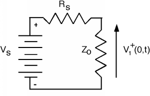
This should look both reasonable and familiar to you. The line and the source resistance are acting as a voltage divider. In fact, Equation \(\PageIndex{4}\) is just the usual voltage divider equation for two resistors in series. Thus, the generator can not tell the difference between a semi-infinite transmission line of characteristic impedance \(Z_{0}\) and a resistor with a resistance of the same value: see Figure \(\PageIndex{3}\).

The positive end of a voltage source v_s is connected in series to a resistor of R_s and then to an impedance of z_0, whose far end connects to the negative end of v_s. There is a voltage drop of V1+ (0, t) across the Z_0 impedance. — Figure \(\PageIndex{3}\): Line is initially a voltage divider!

Have you ever heard of "\(300 \mathrm{~ \Omega}\) twin-lead" or maybe "\(75 \mathrm{~ \Omega}\) co-ax" and wondered why people would want to use wires with such a high resistance value to bring a TV signal to their set? Now you know. The \(300 \mathrm{~ \Omega}\) characterization is not a measure of the resistance of the wire, rather it is a specification of the transmission line's impedance. Thus, if a TV signal coming from your antenna has a value of, say, \(30 \ \mu \mathrm{V}\), and it is being brought down from the roof with \(300 \mathrm{~ \Omega}\) twin-lead, then the current flowing in the wires is \(I = \frac{30 \ \mu \mathrm{V}}{300 \mathrm{~ \Omega}} = 100 \mathrm{~nA}\), which is a very small current indeed!

Why then, did people decide on \(300 \mathrm{~ \Omega}\)? An antenna which is just a half-wavelength long (which turns out to be both a convenient and efficient choice for signals in the \(100 \mathrm{~MHz}\) range, with \(\lambda \simeq 3 \mathrm{~m}\)) acts like a voltage source with a source resistance of about \(300 \mathrm{~ \Omega}\). If you remember from ELEC 242, when we have a source with a source resistance \(R_{s}\) and a load resistor with load resistance value \(R_{L}\) as in Figure \(\PageIndex{4}\), you calculate the power delivered to the load using the following method.

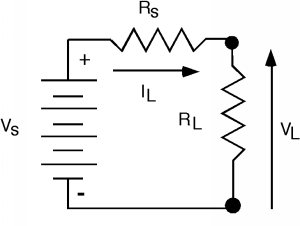
The positive end of a voltage source V_s is connected in series to a resistor R_s and then a resistor R_L, whose far end connects to the negative end of the source. The current exiting the positive end of the voltage source and passing through R_s is labeled I_L, and the voltage drop across R_L is labeled V_L. — Figure \(\PageIndex{4}\): Power transfer to a load

\(P_{L}\), the power in the load, is just product of the voltage across the load times the current through the load. We can use the voltage divider law to find the voltage across \(R_{L}\) and the resistor sum law to find the current through it. \[\begin{array}{l} P_{L} &= V_{L} I_{L} \\ &= \dfrac{R_{L}}{R_{L} + R_{s}} V_{s} \frac{V_{s}}{R_{L} + R_{s}} \\ &= \dfrac{R_{L}}{\left(R_{L} + R_{s}\right)^{2}} V_{s}{ }^{2} \end{array}\] If we take the derivative of Equation \(\PageIndex{5}\) with respect to \(R_{L}\), the load resistor (which we assume we can pick, given some predetermined \(R_{s}\)), we have (ignoring the \(V_{s}{ }^{2}\), \[\frac{\text{d}}{\text{d} R_{L}} \left(P_{L}\right) = \frac{1}{\left(R_{L} + R_{s}\right)^{2}} \frac{2 R_{L}}{\left(R_{L} + R_{s}\right)^{3}} = 0\]

Putting everything on \(\left(R_{L} + R_{s}\right)^{3}\) and then just looking at the numerator: \[R_{L} + R_{s} - 2 R_{L} = 0\]

Which obviously says that for maximum power transfer, you want your load resistor \(R_{L}\) to have the same value as your source resistor \(R_{s}\)! Thus, people came up with the \(300 \mathrm{~\Omega}\) twin lead so that they could maximize the energy transfer between the TV antenna and the transmission line bringing the signal to the TV receiver set. It turns out that for a co-axial transmission line (such as your TV cable), \(75 \mathrm{~\Omega}\) minimizes the signal loss, which is why that value was chosen for CATV.