6.5: Crank Diagram

We actually still have some options open to us. One of the nicest, at least in terms of getting some insight, is called a crank diagram. Note that this equation is a complex equation, which requires us to take the ratio of two complex numbers: $1+{\Gamma }_{\nu }{e}^{-(i2\beta s)}$ and $1-{\Gamma }_{\nu }{e}^{-(i2\beta s)}$.

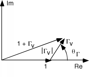
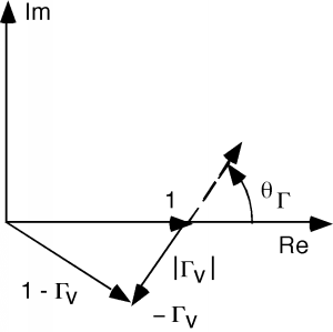
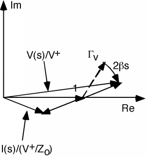
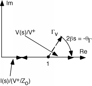
Let's plot these two quantities on the complex plane, starting at $s=0$ (the load end of the line). We can represent ${\Gamma }_{\nu }$, the reflection coefficient, by its magnitude and its phase, which are $\left|{\Gamma }_{\nu }\right|$ and ${\phi }_{\Gamma }$. For the numerator we plot a 1, and then add the complex vector $\Gamma$ which has a length $\left|\Gamma \right|$ and sits at an angle ${\phi }_{\Gamma }$ with respect to the real axis, as shown in Figure \(\PageIndex{1}\). The denominator is just the same thing, except that the \(\Gamma\) vector points in the opposite direction as shown in Figure \(\PageIndex{2}\).

Figure \(\PageIndex{1}\): Plotting $1+{\Gamma }_{\nu }$

Figure \(\PageIndex{2}\): Plotting $1-{\Gamma }_{\nu }$

The top vector is proportional to $V\left(s\right)$ and the bottom vector is proportional to $I\left(s\right)$ Figure \(\PageIndex{3}\). Of course, for $s=0$ we are at the load, so $V\left(s=0\right)=V_L$ and $I\left(s=0\right)=I_L$.

Figure \(\PageIndex{3}\): Another crank diagram showing that $1+{\Gamma }_{\nu }=\frac{V_L}{V^{+}}$ and $1-{\Gamma }_{\nu }=\frac{Z_0{I}_L}{V^{+}}$

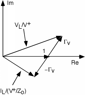
As we move down the line, the two "$\Gamma$" vectors rotate around at a rate of $-2\beta s$as shown in Figure \(\PageIndex{4}\). As they rotate, one vector gets longer and the other gets shorter, and then the opposite occurs. In any event, to get $Z\left(s\right)$ we have to divide the first vector by the second. In general, this is not easy to do, but there are some places where it is not too bad. One of these is when $2\beta s=-{\theta }_{\Gamma }$, which is shown in Figure \(\PageIndex{5}\).

Figure \(\PageIndex{4}\): Rotating the phasors on the crank diagram

Figure \(\PageIndex{5}\): Rotating a crank diagram to a $V_{\max }$

At this point, the voltage vector has rotated around so that it is just lying on the real axis. Obviously its length is now $1+\left|\Gamma \right|$. By the same token, the current vector is also lying on the real axis, and has a length $1-\left|\Gamma \right|$. Dividing one by the other, and multiplying by $Z_0$ gives us $Z\left(s\right)$ at this point.

$$Z\left(s\right)=Z_0\frac{1+\left|{\Gamma }_{\nu }\right|}{1-\left|{\Gamma }_{\nu }\right|}$$

Where is this point, and does it have any special meaning? For this, we need to go back to our expression for $V\left(s\right)$ in this equation.

$$\begin{array}{rcl}\hfill V\left(s\right)& \hfill =\hfill & V^{+}{e}^{i\beta s}(1+{\Gamma }_{\nu }{e}^{-2i\beta s})\hfill \\ \hfill & \hfill =\hfill & V^{+}{e}^{i\beta s}(1+\left|{\Gamma }_{\nu }\right|e^{i({\theta }_{\Gamma }-2\beta s)})\hfill \\ \hfill & \hfill =\hfill & V^{+}{e}^{i\beta s}(1+\left|{\Gamma }_{\nu }\right|e^{i\phi \left(s\right)})\hfill \end{array}$$

where we have substituted $\left|{\Gamma }_{\nu }\right|e^{i\theta }$ for the phasor ${\Gamma }_{\nu }$ and then defined a new angle $\phi \left(s\right)={\theta }_{\Gamma }-2\beta s$.

Now let's find the magnitude of $V\left(s\right)$. To do this we need to square the real and imaginary parts, add them, and then take the square root.

$$\begin{array}{rcl}\hfill \left|V\left(s\right)\right|& \hfill =\hfill & \left|V^{+}\right|(1+\left|{\Gamma }_{\nu }\right|e^{i\phi \left(s\right)})\hfill \\ \hfill & \hfill =\hfill & \left|V^{+}\right|\sqrt{{\left(1+\left|{\Gamma }_{\nu }\right|\cos \left(\phi \left(s\right)\right)\right)}^2+{\left(\left|{\Gamma }_{\nu }\right|\right)}^2{\sin }^2\left(\phi \left(s\right)\right)}\hfill \end{array}$$

so,

$$\left|V\left(s\right)\right|=\left|V^{+}\right|\sqrt{1+2\left|{\Gamma }_{\nu }\right|\cos \left(\phi \left(s\right)\right)+{\left(\left|{\Gamma }_{\nu }\right|\right)}^2{\cos }^2\left(\phi \left(s\right)\right)+{\left(\left|{\Gamma }_{\nu }\right|\right)}^2{\sin }^2\left(\phi \left(s\right)\right)}$$

which, since ${\sin }^2\left(·\right)+{\cos }^2\left(·\right)=1$

$$\left|V\left(s\right)\right|=\left|V^{+}\right|\sqrt{1+{\left(\left|{\Gamma }_{\nu }\right|\right)}^2+2\left|{\Gamma }_{\nu }\right|\cos \left(\phi \left(s\right)\right)}$$

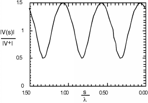
Remember, $\phi \left(s\right)$ is an angle which changes with $s$. In particular, $\phi \left(s\right)={\theta }_{\Gamma }-2\beta s$. Thus, as we move down the line $\left|V\left(s\right)\right|$ will oscillate as $\cos \left(\phi \left(s\right)\right)$ oscillates. A typical plot for $V\left(s\right)$ (for $\left|{\Gamma }_{\nu }\right|=0.5$ and ${\theta }_{\Gamma }={45}^{°}$) is shown below in Figure \(\PageIndex{6}\).

Figure \(\PageIndex{6}\): Standing wave pattern